Triple-Barrier and Meta-Labelling
The primary labeling method used in financial academia is the fixed-time horizon method. While ubiquitous, this method has many faults which are remedied by the triple-barrier method discussed below. The triple-barrier method can be extended to incorporate meta-labeling which will also be demonstrated and discussed below.
Note
Underlying Literature
The following sources describe this method in more detail:
Advances in Financial Machine Learning, Chapter 3 by Marcos Lopez de Prado.
Machine Learning for Asset Managers, Chapter 5 by Marcos Lopez de Prado
Triple-Barrier Method
The idea behind the triple-barrier method is that we have three barriers: an upper barrier, a lower barrier, and a vertical barrier. The upper barrier represents the threshold an observation’s return needs to reach in order to be considered a buying opportunity (a label of 1), the lower barrier represents the threshold an observation’s return needs to reach in order to be considered a selling opportunity (a label of -1), and the vertical barrier represents the amount of time an observation has to reach its given return in either direction before it is given a label of 0. This concept can be better understood visually and is shown in the figure below taken from Advances in Financial Machine Learning:
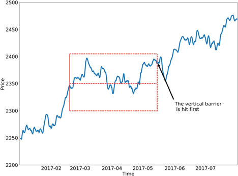
One of the major faults with the fixed-time horizon method is that observations are given a label with respect to a certain threshold after a fixed interval regardless of their respective volatilities. In other words, the expected returns of every observation are treated equally regardless of the associated risk. The triple-barrier method tackles this issue by dynamically setting the upper and lower barriers for each observation based on their given volatilities.
Meta-Labeling
Advances in Financial Machine Learning, Chapter 3, page 50. Reads:
“Suppose that you have a model for setting the side of the bet (long or short). You just need to learn the size of that bet, which includes the possibility of no bet at all (zero size). This is a situation that practitioners face regularly. We often know whether we want to buy or sell a product, and the only remaining question is how much money we should risk in such a bet. We do not want the ML algorithm to learn the side, just to tell us what is the appropriate size. At this point, it probably does not surprise you to hear that no book or paper has so far discussed this common problem. Thankfully, that misery ends here.””
I call this problem meta-labeling because we want to build a secondary ML model that learns how to use a primary exogenous model.
The ML algorithm will be trained to decide whether to take the bet or pass, a purely binary prediction. When the predicted label is 1, we can use the probability of this secondary prediction to derive the size of the bet, where the side (sign) of the position has been set by the primary model.
Tip
- Pull inspiration on Meta-Labeling from these papers:
How to use Meta-Labeling
Binary classification problems present a trade-off between type-I errors (false positives) and type-II errors (false negatives). In general, increasing the true positive rate of a binary classifier will tend to increase its false positive rate. The receiver operating characteristic (ROC) curve of a binary classifier measures the cost of increasing the true positive rate, in terms of accepting higher false positive rates.
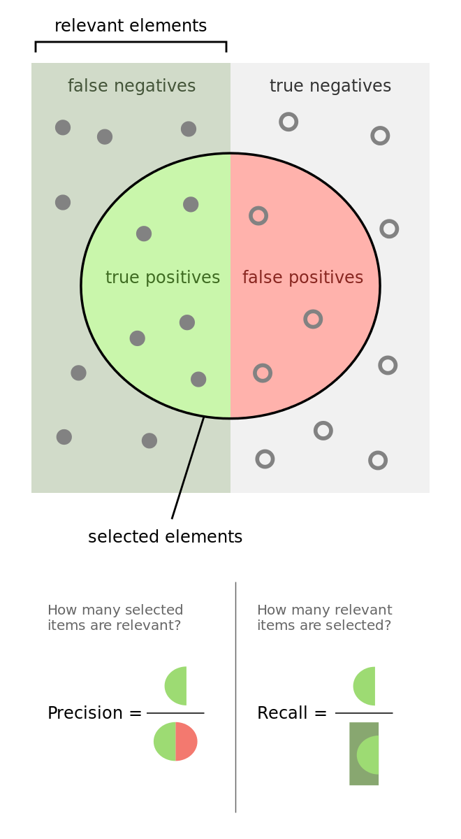
The image illustrates the so-called “confusion matrix.” On a set of observations, there are items that exhibit a condition (positives, left rectangle), and items that do not exhibit a condition (negative, right rectangle). A binary classifier predicts that some items exhibit the condition (ellipse), where the TP area contains the true positives and the TN area contains the true negatives. This leads to two kinds of errors: false positives (FP) and false negatives (FN). “Precision” is the ratio between the TP area and the area in the ellipse. “Recall” is the ratio between the TP area and the area in the left rectangle. This notion of recall (aka true positive rate) is in the context of classification problems, the analogous to “power” in the context of hypothesis testing. “Accuracy” is the sum of the TP and TN areas divided by the overall set of items (square). In general, decreasing the FP area comes at a cost of increasing the FN area, because higher precision typically means fewer calls, hence lower recall. Still, there is some combination of precision and recall that maximizes the overall efficiency of the classifier. The F1-score measures the efficiency of a classifier as the harmonic average between precision and recall.
Meta-labeling is particularly helpful when you want to achieve higher F1-scores. First, we build a model that achieves high recall, even if the precision is not particularly high. Second, we correct for the low precision by applying meta-labeling to the positives predicted by the primary model.
Meta-labeling will increase your F1-score by filtering out the false positives, where the majority of positives have already been identified by the primary model. Stated differently, the role of the secondary ML algorithm is to determine whether a positive from the primary (exogenous) model is true or false. It is not its purpose to come up with a betting opportunity. Its purpose is to determine whether we should act or pass on the opportunity that has been presented.
Meta-labeling is a very powerful tool to have in your arsenal, for four additional reasons. First, ML algorithms are often criticized as black boxes. Meta-labeling allows you to build an ML system on top of a white box (like a fundamental model founded on economic theory). This ability to transform a fundamental model into an ML model should make meta-labeling particularly useful to “quantamental” firms. Second, the effects of overfitting are limited when you apply metalabeling, because ML will not decide the side of your bet, only the size. Third, by decoupling the side prediction from the size prediction, meta-labeling enables sophisticated strategy structures. For instance, consider that the features driving a rally may differ from the features driving a sell-off. In that case, you may want to develop an ML strategy exclusively for long positions, based on the buy recommendations of a primary model, and an ML strategy exclusively for short positions, based on the sell recommendations of an entirely different primary model. Fourth, achieving high accuracy on small bets and low accuracy on large bets will ruin you. As important as identifying good opportunities is to size them properly, so it makes sense to develop an ML algorithm solely focused on getting that critical decision (sizing) right. We will retake this fourth point in Chapter 10. In my experience, meta-labeling ML models can deliver more robust and reliable outcomes than standard labeling models.
Model Architecture
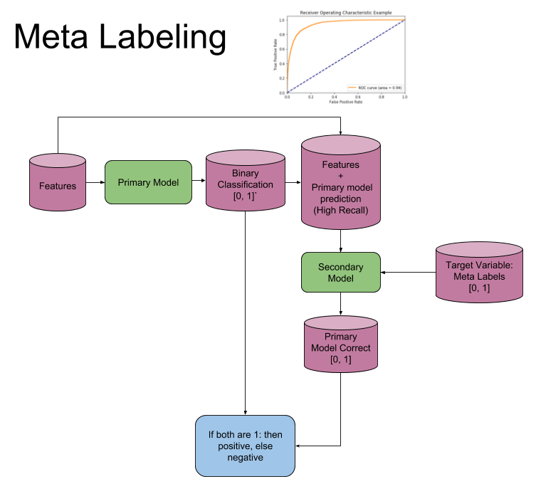
The following image explains the model architecture. The first step is to train a primary model (binary classification). Second a threshold level is determined at which the primary model has a high recall, in the coded example you will find that 0.30 is a good threshold, ROC curves could be used to help determine a good level. Third the features from the first model are concatenated with the predictions from the first model, into a new feature set for the secondary model. Meta Labels are used as the target variable in the second model. Now fit the second model. Fourth the prediction from the secondary model is combined with the prediction from the primary model and only where both are true, is your final prediction true. I.e. if your primary model predicts a 3 and your secondary model says you have a high probability of the primary model being correct, is your final prediction a 3, else not 3.
Implementation
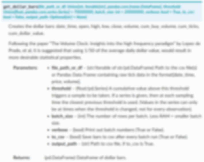
The following functions are used for the triple-barrier method which works in tandem with meta-labeling.
Note
For this section we retained the books original function names, so that the user could have a smoother journey.

Example
Suppose we use a mean-reverting strategy as our primary model, giving each observation a label of -1 or 1. We can then use meta-labeling to act as a filter for the bets of our primary model.
Assuming we have a pandas series with the timestamps of our observations and their respective labels given by the primary model, the process to generate meta-labels goes as follows.
Once we have computed the daily volatility along with our vertical time barriers and have downsampled our series using the CUSUM filter, we can use the triple-barrier method to compute our meta-labels by passing in the side predicted by the primary model.
As can be seen above, we have scaled our lower barrier and set our minimum return to 0.005.
Warning
The biggest mistake we see users making here is that they change the daily targets and min_ret values to get more observations, since ML models require a fair amount of data. This is the wrong approach!
Please visit the Seven-Point Protocol under the Backtest Overfitting Tools section to learn more about how to think about features and outcomes.
Meta-labels can then be computed using the time that each observation touched its respective barrier.
This example ends with creating the meta-labels. To see a further explanation of using these labels in a secondary model to help filter out false positives, see the research notebooks below.
Blog Posts
Does Meta Labeling Add to Signal Efficacy?
Successful and long-lasting quantitative research programs require a solid foundation that includes procurement and curation of data, creation of building blocks for feature engineering, state of the art methodologies, and backtesting. In this project we explore an example of applying meta labeling to high quality S&P500 EMini Futures data and create a python package (MlFinLab) that is based on the work of Dr. Marcos Lopez de Prado in his book ‘Advances in Financial Machine Learning’. Dr. de Prado’s book provides a guideline for creating a successful platform. We also implement a Trend Following and Mean-reverting Bollinger band based trading strategies. Our results confirm the fact that a combination of event-based sampling, triple-barrier method and meta labeling improves the performance of the strategies.
Meta Labeling (A Toy Example)
This blog post investigates the idea of Meta Labeling and tries to help build an intuition for what is taking place. The idea of meta-labeling is first mentioned in the textbook Advances in Financial Machine Learning by Marcos Lopez de Prado and promises to improve model and strategy performance metrics by helping to filter-out false positives.
We make use of a computer vision problem known as the MNIST handwritten digit classification. By using of a non-financial timeseries data set we can illustrate the components that make up meta labeling more clearly. Lets begin!
Research Notebook
The following research notebooks can be used to better understand the triple-barrier method and meta-labeling
Meta-Labeling Toy Example