Note
The following implementations and documentation, closely follows the lecture notes from Cornell University, by Marcos Lopez de Prado: Codependence (Presentation Slides).
Correlation-Based Metrics
Note
Underlying Literature
The following sources elaborate extensively on the topic:
Codependence (Presentation Slides) by Marcos Lopez de Prado.
Measuring and testing dependence by correlation of distances by Székely, G.J., Rizzo, M.L. and Bakirov, N.K.
Introducing the discussion paper by Székely and Rizzo by Michael A. Newton.
Building Diversified Portfolios that Outperform Out-of-Sample by Marcos Lopez de Prado.
Kullback-Leibler distance as a measure of the information filtered from multivariate data. by Tumminello, M., Lillo, F. and Mantegna, R.N.
Distance Correlation
Distance correlation can capture not only linear association but also non-linear variable dependencies which Pearson correlation can not. It was introduced in 2005 by Gábor J. Szekely and is described in the work “Measuring and testing independence by correlation of distances”. It is calculated as:
Where \(dCov[X, Y]\) can be interpreted as the average Hadamard product of the doubly-centered Euclidean distance matrices of \(X, Y\). (Cornell lecture slides, p.7)
Values of distance correlation fall in the range:
Distance correlation is equal to zero if and only if the two variables are independent (in contrast to Pearson correlation that can be zero even if the variables are dependant).
As shown in the figure below, distance correlation captures the nonlinear relationship.
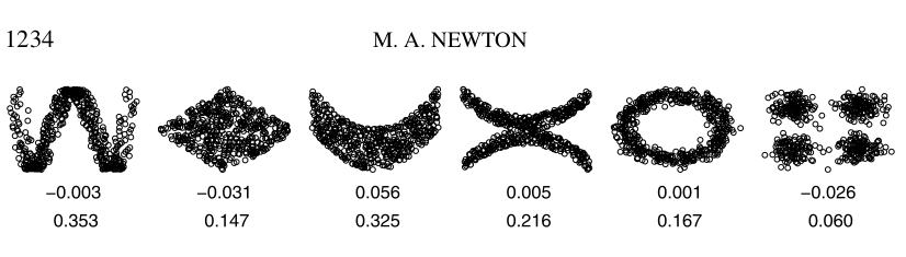
The numbers in the first line are Pearson correlation values and the values in the second line are Distance correlation values. This figure is from “Introducing the discussion paper by Székely and Rizzo” by Michale A. Newton. It provides a great overview for readers.
Implementation
Standard Angular Distance
Angular distance is a slight modification of the Pearson correlation coefficient which satisfies all distance metric conditions. This measure is known as the angular distance because when we use covariance as an inner product, we can interpret correlation as \(cos\theta\).
A proof that angular distance is a true metric can be found in the work by Lopez de Prado Building Diversified Portfolios that Outperform Out-of-Sample:
“Angular distance is a linear multiple of the Euclidean distance between the vectors \(\{X, Y\}\) after z-standardization, hence it inherits the true-metric properties of the Euclidean distance.”
According to Lopez de Prado:
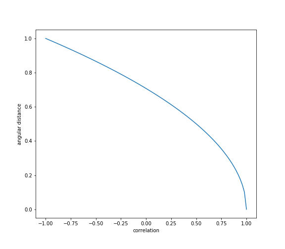
“The [standard angular distance] metric deems more distant two random variables with negative correlation than two random variables with positive correlation”.
“This property makes sense in many applications. For example, we may wish to build a long-only portfolio, where holdings in negative-correlated securities can only offset risk, and therefore should be treated as different for diversification purposes”.
Formula used to calculate standard angular distance:
where \(\rho[X,Y]\) is Pearson correlation between the vectors \(\{X, Y\}\) .
Values of standard angular distance fall in the range:
The angular distance satisfies all the conditions of a true metric, (Lopez de Prado, 2020.)
Implementation
Absolute Angular Distance
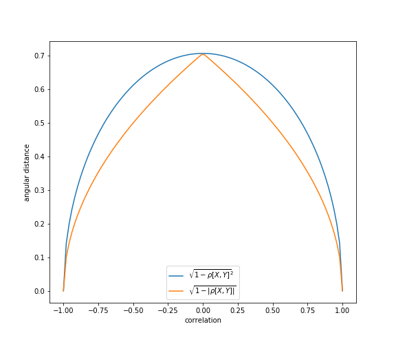
This modification of angular distance uses an absolute value of Pearson correlation in the formula.
This property assigns small distance to elements that have a high negative correlation. According to Lopez de Prado, this is useful because “in long-short portfolios, we often prefer to consider highly negatively-correlated securities as similar, because the position sign can override the sign of the correlation”.
Formula used to calculate absolute angular distance:
where \(\rho[X,Y]\) is Pearson correlation between the vectors \(\{X, Y\}\) .
Values of absolute angular distance fall in the range:
In some financial applications, it makes more sense to apply a modified definition of angular distance, such that the sign of the correlation is ignored, (Lopez de Prado, 2020)
Implementation
Squared Angular Distance
Squared angular distance uses the squared value of Pearson correlation in the formula and has similar properties to absolute angular distance. The only difference is that a higher distance is assigned to the elements that have a small absolute correlation.
Formula used to calculate squared angular distance:
where \(\rho[X,Y]\) is Pearson correlation between the vectors \(\{X, Y\}\) .
Values of squared angular distance fall in the range:
Implementation
Kullback-Leibler Distance
The Kullback-Leibler distance is a measure of distance between two probability densities, say p and q, which is defined as
Where \(E_p[.]\) indicates the expectation value with respect to the probability density \(p\). Here we consider the Kullback-Leibler distance between multivariate Gaussian random variables (aka. Correlation matrices).
Given two positive definite correlation matrices \(C_1\) and \(C_2\) associated with random variable \(X\), we can compute their probability density functions to \(P(C_1,X)\) and \(P(C_1,X)\) resulting in the following formula
where \(n\) is the dimension of the space spanned by \(X\), and \(|C|\) indicates the determinant of \(C\)
The Kullback-Leibler distance can be used to measure the stability of filtering/de-noising procedures with respect to statistical uncertainty.
Tip
It is worth noting that the Kullback-Leibler distance takes naturally into account the statistical nature of correlation matrices which is uncommon with other measures of distance between matrices such as the Frobenius distance which is based on the iso-morphism between the matrices space and the vectors space. For more information on using the Kullback-Leibler distance to measure the statistical uncertainty of correlation matrices check out Michele Tumminello’s research paper.
Implementation
Norm Distance
A Norm is a function that takes a random variable and returns a value(Norm Distance) that satisfies certain properties pertaining to scalability and additivity.
The \(L\) norms are the most common type of norms. They use the same logic behind the SRSS (Square Root of the Sum of Squares)
where \(r\) is a positive integer. The Euclidean norm is by far the most commonly used norm on multi-dimensional variables with \(r = 2\) which makes the Euclidean norm an \(L^2\) type norm.
Implementation
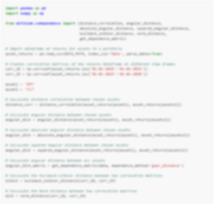
Examples
The following examples show how the described above correlation-based metrics can be used on real data: