Average Linkage Minimum Spanning Tree (ALMST)
Average Linkage Minimum Spanning Tree (ALMST) shows better results in recognising the economic sectors and sub-sectors than the Minimum Spanning Tree (Tumminello et al. 2007). The ALMST, as defined by Tumminello et al. (2007), is a variation of the MST.
Just as the MST is associated with the Single Linkage Clustering Algorithm (SCLA), the ALMST is based on the UPGMA (unweighted pair group method with arithmetic mean) algorithm for hierarchal clustering. This is also known as Average Linkage Cluster Algorithm (ALCA) method. The UPGMA method is frequently used in biology for phylogenetic tree as a diagrammatic representation of the evolutionary relatedness between organisms. A step by step example of UPGMA or ALCA method for trees can be found here.
Note
Underlying Literature
The following sources describe this method in more detail:
Spanning trees and bootstrap reliability estimation in correlation-based networks by M. Tumminello, C. Coronnello, F. Lillo, S. Micciche, R. N. Mantegna.
ALMST
ALMST vs. MST
Instead of choosing the next edge by the minimum edge (distance based MST), the next edge is chosen by the minimum average distance between two existing clusters. Tumminello et al. (2007) give an example MST algorithm to show how the ALMST algorithm differs from the MST algorithm.
Where \(g\) is the graph, \(S_{i}\) is the set of vertices, \(n\) is the number of elements, \(C\) is the correlation matrix of elements \(ρ_{ij}\), connected component of a graph \(g\) containing a given vertex \(i\). The starting point of the procedure is an empty graph \(g\) with \(n\) vertices.
Set \(Q\) as the matrix of elements \(q_{ij}\) such that \(Q = C\), where \(C\) is the estimated correlation matrix.
Select the maximum correlation \(q_{hk}\) between elements belonging to different connected components \(S_{h}\) and \(S_{k}\) in \(g^{2}\).
Find elements \(u\), \(p\) such that \(p_{up} = \max\{{\rho_{ij}}, \forall i \in S_{h}\) and \(\forall j \in S_{k} \}\)
Add to \(g\) the link between elements \(u\) and \(p\) with weight \(\rho_{up}\). Once the link is added to \(g\), \(u\) and \(p\) will belong to the same connected component \(S = S_{h} \cup S_{k}\).
Redefine the matrix \(Q\):
If \(g\) is still a disconnected graph then go to step (2) else stop.
This is the case for a correlation matrix (taking the maximum correlation value for the MST edges).
However, for distance matrices, the MST algorithm orders the edges by the minimum distance, by replacing step (5) with:
By replacing eq. in step (5) with
we obtain an algorithm performing the ALCA. We call the resulting tree \(g\) an ALMST.
User Interface
The ALMST can be generated in the same way as the MST, but by creating an ALMST class object instead. Since MST and ALMST are both subclasses of Graph, MST and ALMST are the input to the initialisation method of class Dash. However, the recommended way to create visualisations, is to use the methods from visualisations file, unless you would like to input a custom matrix.
Creating the ALMST visualisation is a similar process to creating the MST. You can replace:

With:
This creates the ALMST object containing self.graph as the graph of the ALMST. The ALMST object can then be inputted to the Dash interface.
Implementation

ALMST Algorithms
When you initialise the ALMST object, the ALMST is generated and stored as attribute an self.graph. Kruskal’s algorithms is used as a default.
To use Prim’s algorithm, pass the string ‘prim’.
Example Code
Customizing the Graphs
To further customize the ALMST when it is displayed in the Dash UI, you can add colours and change the sizes to represent for example industry groups and market cap of stocks.
These features are optional and only work for the Dash interface (not the comparison interface). As the comparison interface, highlights the central nodes (with degree greater than or equal to 5).
Adding Colours to Nodes
The colours can be added by passing a dictionary of group name to list of node names corresponding to the nodes input. You then pass the dictionary to the set_node_groups method.
Adding Sizes to Nodes
The sizes can be added in a similar manner, via a list of numbers which correspond to the node indexes. The UI of the graph will then display the nodes indicating the different sizes.
Comparison Interface
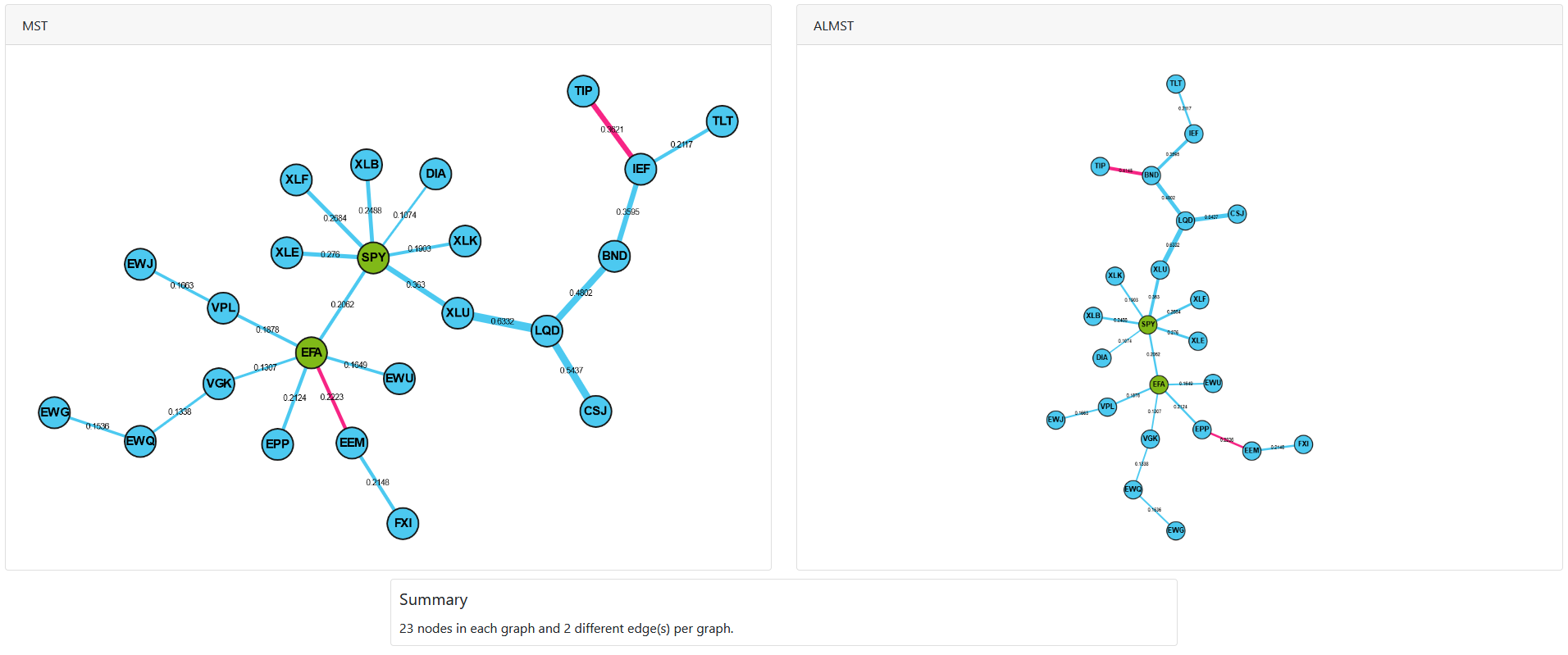
ALMST and MST can be compared easily using the DualDashGraph interface, where you can see the MST and ALMST side by side. You can also create the dual interface using generate_mst_almst_comparison method in the Visualisations section. This is the recommended way as it reduces the number of steps needed to create the interface.