History Weighted Regression
Intuitively, when we look at history data to make a reasonable guess of the current situation, we tend to at first identify similar cases to our current situation. For example, say we are trying to predict a stock price with some companies’ fundamental data (could be more than 1 company). Then amongst those similar cases, we tend to take a deeper look at those that are farther away from the historical mean, because they usually bear more interesting information, and the average cases are plenty and they could just fluctuate due to noise.
Note
This documentation is based on the following three papers written by Megan Szasonis, Mark Kritzman and David Turkington.
We mostly implement by choosing the consensus used in [Relevance] to be more consistent in notations.
Introduction and Ideas
The history weighed regression method proposed by Megan Szasonis, Mark Kritzman and David Turkington, has the following three key features, as written in [Addition by Subtraction]:
The prediction from a linear regression equation is mathematically equivalent to a weighted average of the past values of the dependent variable, in which the weights are the relevance of the independent observations.
Relevance within this context is defined as the sum of statistical similarity and informativeness, both of which are defined as Mahalanobis distances.
Together, these features allow researchers to censor less relevant observations and derive more reliable predictions of the dependent variable.
Simply speaking, this is a method that selects a subsample based on how relevant each history instance in the training set is to our test instance, and run prediction on the subsample (i.e., a given percentage of all events ranked by relevance). Moreover, when one chooses to use run prediction over all events (i.e., 100% of all events ranked by relevance), this method’s result coincide with OLS.
Definitions and Concepts
Note
To keep the notations consistent in this document, we assume all vectors are column vectors (the common way in linear algebra textbooks, though not in machine learning books), and an n-by-k matrix storing data has n instances and k features (the usual way people implement in pandas.).
Mahalanobis Distances
Suppose we have an N-by-k data matrix \(X\), with \(N\) many instances and \(k\) features. Think about \(X\) as our training set. Then we can calculate the features covariance matrix (k-by-k) as
Assuming the \(\Omega\) is symmetric positive definite (i.e., no 0 variances), then we can calculate the Fisher information matrix \(\Omega^{-1}\) (though strictly speaking it is only true asymptotically in the frequentist sense, but we borrow the name here anyway).
The Mahalanobis Distance of two instances \(x_i, x_j\) are defined as follows in the quadratic form:
because \(\Omega^{-1}\) is also symmetric and positive definite.
Intuitively, because \(\Omega\) records the variances among our data for each feature around the mean, \(\Omega^{-1}\) records how tight the training data are for each feature around the mean. Therefore, \(x^T \Omega^{-1} x\) is the amount of information along the direction \(x\): The larger the value, the larger the amount of information. Hence \(d_M(x_i, x_j)\) quantifies the amount of information given the training data between two specific instances \((x_i, x_j)\), and the two instances are arbitrary as they do not have to all come from training set or test set, though we often assume \(x_i\) to be a past instance and \(x_j\) to be a test instance for interpretability.
Similarity
Now we define the similarity between two instances \((x_i, x_j)\) as the negative of their Mahalanobis distance:
Trivially, when \(x_i = x_j\) then they are the most similar pair and the similarity will become 0, the largest value. This quantity measures how similar two instances are, based on our training set. The larger the value, the more similar they are, and as a result the less information one can get.
Informativeness
Remember that \(x^T \Omega^{-1} x\) is the amount of information along the direction \(x\) away from the mean, we can therefore define the informativeness as below:
where \(\bar{x}\) is the mean of our training data \(X\) for each feature. The larger the value, the less similar \(x_i\) is to the mean, and therefore the more information it brings.
Note
Similarity and informativeness are addressing different aspects of the data. They are in some sense the opposite of each other but with some nuances here: similarity is used to measure between two instances whereas informativeness is used to measure between one instance to the training data. We will combine the two together to form the key value for the history weighted regression method called relevance.
Relevance and Subsample
Now we can define the relevance value between two instances \((x_i, x_t)\) as follows:
Relevance is interpreted as the sum of similarity and informativeness for \((x_i, x_t)\), where \(x_i\) is in the training set, and \(x_t\) is a test instance. Intuitively, when the in-sample instance and the test instance pair \((x_i, x_t)\) are similar and give great information, their relevance value will be greater.
Indeed, relevance is one of the values to quantify the thought process we had in the beginning for guessing the stock’s price using companies fundamental data. The figure below gives a good explanation on relevance. Note that the two history events are on their elliptical orbits of fixed amounts of informativeness.
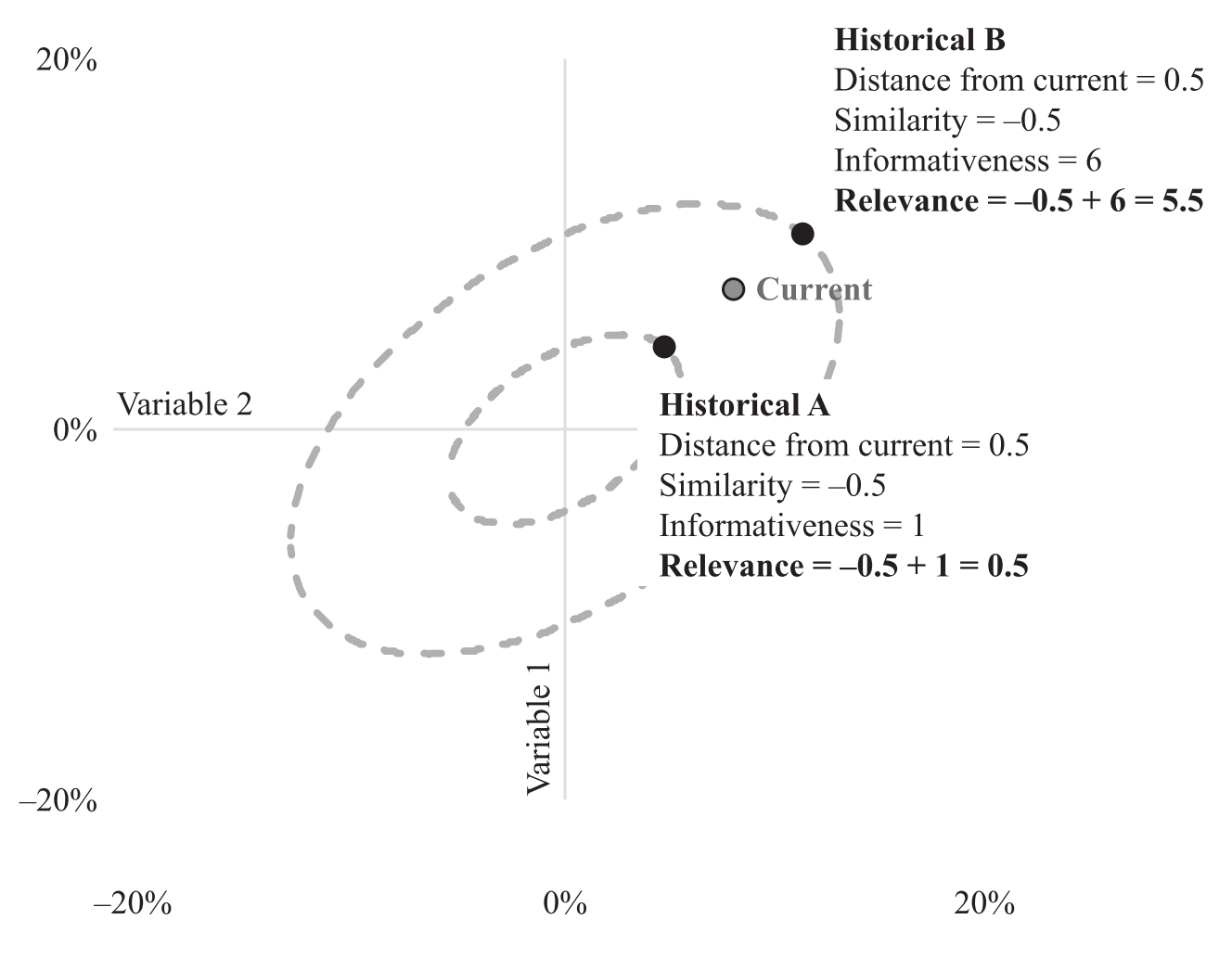
An illustration of the relationship between similarity, informativeness and relevance. We choose the historical event B to be more relevant to our current case than event A. (Figure from [Addition by Subtraction])
Prediction
Now we have a instance in independent variable \(x_t\), we aim to make a prediction \(\hat{y}_t\) based on \(x_t\). Say the training data for independent variable is in the matrix N-by-K \(X\) and the dependent variable is in the N-by-1 vector \(Y\).
Workflow
Calculate all relevance between \(x_t\) and each row of \(X\): \(r_{it}\) where \(i = 1,\cdots, N\).
Rank all the instances in relevance and pick the instances in top \(q \in (0, 1]\) quantiles to form a subsample with \(n\) instances.
Make prediction using the formula
\[\hat{y}_t = \bar{y} + \frac{1}{n-1} \sum_{i=1}^n r_{it} (y_i - \bar{y})\]where \(\bar{y}\) is the subsample average of the dependent variable.
We can read the formula above in two parts: First, when no information is given about \(X\), the best prediction we can formulate for the unknown \(y_t\) is \(\bar{y}\). The second part can be interpreted as a weighted average by relevance of historical deviations for the dependent variable, and the weights are computed by \(x_i, x_t, i=1, \cdots, n\).
Tip
It is a good practice to rescale \(X\) for each feature, for example, by the number of standard deviations from its mean. This will in general produce a covariance matrix with smaller condition numbers, and thus for the Fisher information matrix since their condition numbers are equal. A smaller condition number is more stable numerically in the calculation, especially when we initially calculate the inverse of the covariance matrix. Because every step for prediction is linear, the final prediction will not change, and do not need to re-scale.
Connection with OLS
We aim to show that, when we do not reduce to a subsample (i.e., \(q=1\) or equivalently \(n=N\)), then the above prediction is identical with prediction given by OLS. First, without loss of generality assume \(X\) and \(Y\) have means of 0. Then plug
into the prediction formula, we get
Where \(X_{sub}\) and \(Y_{sub}\) are the associated subsamples selected by relevance with \(x_t\). Since we assume \(q=1\), equivalently \(n=N\), we have
which is the formula for OLS.
Summary and Comments
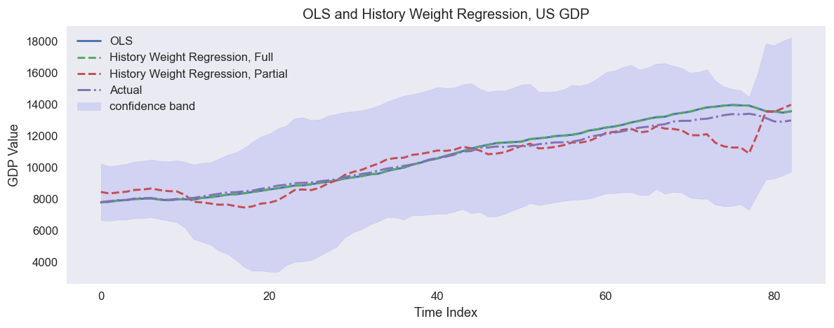
An example of predicting US quarterly GDP in 1988-2009 using quarterly fundamental data from 1959-1987: real personal consumption expenditures, real federal consumption expenditures & gross investment, unemployment rate and M1 (seasonally adjusted). The full sample regression collides with OLS.
Most of the summaries and comments below are taken directly from the three articles, though may be worded slightly differently.
The prediction from a linear regression equation is mathematically equivalent to a weighted average of past values of the dependent variable in which the weights are the relevance of the independent variables.
This equivalence allows one to form a relevance-weighted prediction of the dependent variable by using only a subsample of relevant observations. This approach is called partial sample regression.
Like partial sample regression, an event study separates relevant observations from non-relevant observations, but it does so by identification rather than mathematically.
We should also note that our approach is different from weighted least squares regression, which uses fixed weights regardless of the data point being predicted and applies the weights to calculate the covariance matrix among predictors.
This regression method is different from performing separate regressions on subsamples of the most relevant observations; in a separate regression approach, the covariance matrix used for estimation would also be based on the subsample, whereas we always use the full-sample covariance matrix.
The calculation is invariant under linear re-scale of \(X\). Rescale to get a better condition number for \(\Omega^{-1}\).
This method is conceptually different from PCA, where feature importance is considered. This regression method considers importance in instances, not features. However, one can combine the PCA transformation and the partial sample regression, and if all principal components are considered, the prediction result will be identical compared to directly working with \(X\).
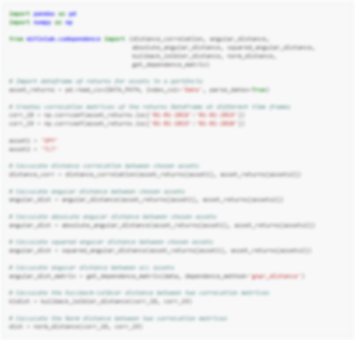
Implementation
Example
Research Notebooks
The following research notebook can be used to better understand the History Weighted Regression.