Structural Breaks
This implementation is based on Chapter 17 of the book Advances in Financial Machine Learning. Structural breaks, like the transition from one market regime to another, represent the shift in the behaviour of market participants.
The first market participant to notice the changes in the market can adapt to them before others and, consequently, gain an advantage over market participants who have not yet noticed market regime changes.
To quote Marcos Lopez de Prado, “Structural breaks offer some of the best risk/rewards”.
We can classify the structural break in two general categories:
CUSUM tests: These test whether the cumulative forecasting errors significantly deviate from white noise.
Explosiveness tests: Beyond deviation from white noise, these test whether the process exhibits exponential growth or collapse, as this is inconsistent with a random walk or stationary process, and it is unsustainable in the long run.
Note
Underlying Literature
The following sources elaborate extensively on the topic:
Advances in Financial Machine Learning, Chapter 17 by Marcos Lopez de Prado. Describes structural breaks in more detail.
Testing for Speculative Bubbles in Stock Markets: A Comparison of Alternative Methods by Ulrich Homm and Jorg Breitung. Explains the Chu-Stinchcombe-White CUSUM Test in more detail.
Tests of Equality Between Sets of Coefficients in Two Linear Regressions by Gregory C. Chow. A work that inspired a family of explosiveness tests.
CUSUM tests
Chu-Stinchcombe-White CUSUM Test on Levels
We are given a set of observations \(t = 1, ... , T\) and we assume an array of features \(x_{i}\) to be predictive of a value \(y_{t}\) .
Authors of the Testing for Speculative Bubbles in Stock Markets: A Comparison of Alternative Methods paper suggest assuming \(H_{0} : \beta_{t} = 0\) and therefore forecast \(E_{t-1}[\Delta y_{t}] = 0\). This allows working directly with \(y_{t}\) instead of computing recursive least squares (RLS) estimates of \(\beta\) .
As \(y_{t}\) we take the log-price and calculate the standardized departure of \(y_{t}\) relative to \(y_{n}\) (CUSUM statistic) with \(t > n\) as:
With the \(H_{0} : \beta_{t} = 0\) hypothesis, \(S_{n, t} \sim N[0, 1]\) .
We can test the null hypothesis comparing CUSUM statistic \(S_{n, t}\) with critical value \(c_{\alpha}[n, t]\), which is calculated using a one-sided test as:
The authors in the above paper have derived using Monte Carlo method that \(b_{0.05} = 4.6\) .
The disadvantage is that \(y_{n}\) is chosen arbitrarily, and results may be inconsistent due to that. This can be fixed by estimating \(S_{n, t}\) on backward-shifting windows \(n \in [1, t]\) and picking:
Implementation

Explosiveness tests
Chow-Type Dickey-Fuller Test
The Chow-Type Dickey-Fuller test is based on an \(AR(1)\) process:
where \(\varepsilon_{t}\) is white noise.
This test is used for detecting whether the process changes from the random walk (\(\rho = 1\)) into an explosive process at some time \(\tau^{*}T\), \(\tau^{*} \in (0,1)\), where \(T\) is the number of observations.
So, the hypothesis \(H_{0}\) is tested against \(H_{1}\):
To test the hypothesis, the following specification is being fit:
So, the hypothesis tested are now transformed to:
And the Dickey-Fuller-Chow(DFC) test-statistics for \(\tau^*\) is:
As described in the Advances in Financial Machine Learning:
The first drawback of this method is that \(\tau^{*}\) is unknown, and the second one is that Chow’s approach assumes that there is only one break and that the bubble runs up to the end of the sample.
To address the first issue, in the work Tests for Parameter Instability and Structural Change With Unknown ChangePoint available here, Andrews proposed to try all possible \(\tau^{*}\) in an interval \(\tau^{*} \in [\tau_{0}, 1 - \tau_{0}]\)
For the unknown \(\tau^{*}\) the test statistic is the Supremum Dickey-Fuller Chow which is the maximum of all \(T(1 - 2\tau_{0})\) values of \(DFC_{\tau^{*}}\) :
To address the second issue, the Supremum Augmented Dickey-Fuller test was introduced.
Implementation
Supremum Augmented Dickey-Fuller
This test was proposed by Phillips, Shi, and Yu in the work Testing for Multiple Bubbles: Historical Episodes of Exuberance and Collapse in the S&P 500 available here. The advantage of this test is that it allows testing for multiple regimes switches (random walk to bubble and back).
The test is based on the following regression:
And, the hypothesis \(H_{0}\) is tested against \(H_{1}\):
The Supremum Augmented Dickey-Fuller fits the above regression for each end point \(t\) with backward expanding start points and calculates the test-statistic as:
where \(\hat\beta_{t_0,t}\) is estimated on the sample from \(t_{0}\) to \(t\), \(\tau\) is the minimum sample length in the analysis, \(t_{0}\) is the left bound of the backwards expanding window, \(t\) iterates through \([\tau, ..., T]\) .
In comparison to SDFC, which is computed only at time \(T\), the SADF is computed at each \(t \in [\tau, T]\), recursively expanding the sample \(t_{0} \in [1, t - \tau]\) . By doing so, the SADF does not assume a known number of regime switches.
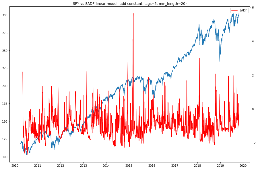
Image showing SADF test statistic with 5 lags and linear model. The SADF line spikes when prices exhibit a bubble-like behavior, and returns to low levels when the bubble bursts.
The model and the add_const parameters of the get_sadf function allow for different specifications of the regression’s time trend component.
Linear model (model=’linear’) uses a linear time trend:
Quadratic model (model=’quadratic’) uses a second-degree polynomial time trend:
Adding a constant (add_const=True) to those specifications results in:
and
respectively.
Implementation
The function used in the SADF Test to estimate the \(\hat\beta_{t_0,t}\) is:
Tip
Advances in Financial Machine Learning book additionally describes why log prices data is more appropriate to use in the above tests, their computational complexity, and other details.
The SADF also allows for explosiveness testing that doesn’t rely on the standard ADF specification. If the process is either sub- or super martingale, the hypotheses \(H_{0}: \beta = 0, H_{1}: \beta \ne 0\) can be tested under these specifications:
Polynomial trend (model=’sm_poly_1’):
Polynomial trend (model=’sm_poly_2’):
Exponential trend (model=’sm_exp’):
Power trend (model=’sm_power’):
Again, the SADF fits the above regressions for each end point \(t\) with backward expanding start points, but the test statistic is taken as an absolute value, as we’re testing both the explosive growth and collapse. This is described in more detail in the Advances in Financial Machine Learning book p. 260.
The test statistic calculated (SMT for Sub/Super Martingale Tests) is:
From the book:
Parameter phi in range (0, 1) can be used (phi=0.5) to penalize large sample lengths ( “this corrects for the bias that the \(\hat\sigma_{\beta_{t_0, t}}\) of a weak long-run bubble may be smaller than the \(\hat\sigma_{\beta_{t_0, t}}\) of a strong short-run bubble, hence biasing method towards long-run bubbles” ):
Example
Presentation Slides

Note
pg 1-14: Structural Breaks
pg 15-24: Entropy Features
pg 25-37: Microstructural Features