Noise Reduction
Note
Underlying Literature
The following material and code implementations have been adapted from:
Kinetic Component Analysis by Marcos Lopez de Prado & Riccardo Rebonato.
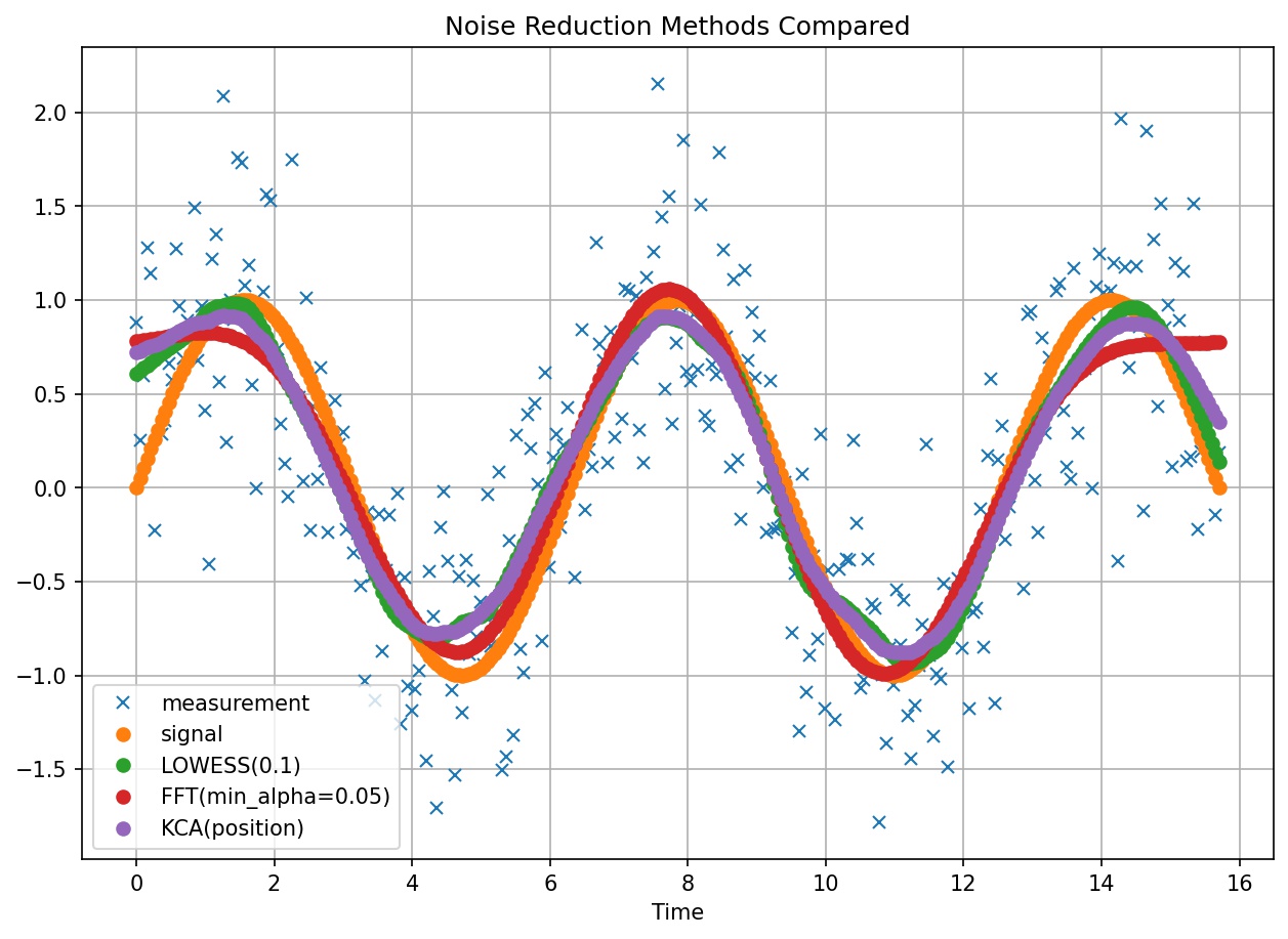
Comparison of noise reduction methods against a sine wave signal with a random component of gaussian noise.
In the paper referred above, the authors, Marcos Lopez de Prado and Riccardo Rebonato, explore different signal processing techniques against their newly proposed Kinetic Component Analysis (KCA). Their proposed technique decomposes a signal into three hidden components, intuitively associated to position, velocity and acceleration.
Any economic observable id defined as \(P(t)\), which may represent prices, rates, yields, or any other asset value quotation,
where \(p(t)\) is defined as the fundamental component and \(h(t)\) as a source of noise.
As markets organically evolve over time, these economic observables acquire a noisy component \(h(t)\), as a result hiding the fundamental component \(p(t)\), which is considered to be a more accurate feature of the economic observable \(P(t)\).
The noise reduction methods in the paper aim to reduce the amount of noise in the economic observable of interest in order to obtain a smoother feature given by the fundamental component \(p(t)\).
Below are reference implementations for the methods discussed in the paper. All the noise reduction methods inherit a
common NoiseReductionMethod class. Below we illustrate some examples of the introduced methods to the
MlFinLab package.
The noise reduction methods implemented expect a pandas.DataFrame as a time series with the “noisy signal” as the first column of the dataframe. To run the core noise reduction algorithm on the noisy signal use generate_signal() method. For other provided class methods, see corresponding implementation reference sections.
Kinetic Component Analysis (KCA)
Overview
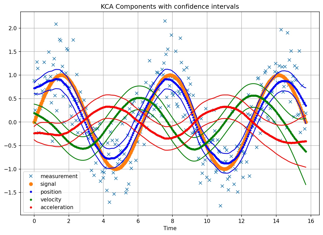
Illustration shows KCA components with confidence intervals over noisy measurements and original sine wave signal.
The authors present Kinetic Component Analysis, as a state-space application that extracts the signal from a series of noisy measurements by applying a Kalman Filter on a Taylor expansion of a stochastic process.
The value of KCA against other methods explored in the paper is that it provides the following unique capabilities:
Band estimates (e.g. confidence intervals) in addition to point estimates
Additional information via decomposition of three hidden components (position, velocity, acceleration)
Forecasting capabilities
Implementation
Important
The greater the value of seed the more likely we are to overfit. This value indicates to the model that a greater proportion of noise comes from the states rather than the measurements (observations).
The authors recommned to try different values of seed that is consistant with your understanding of the system in question.
Generally, opt for lower values of seed to avoid overfitting.
Example
Fast Fourier Transform (FFT)
Overview
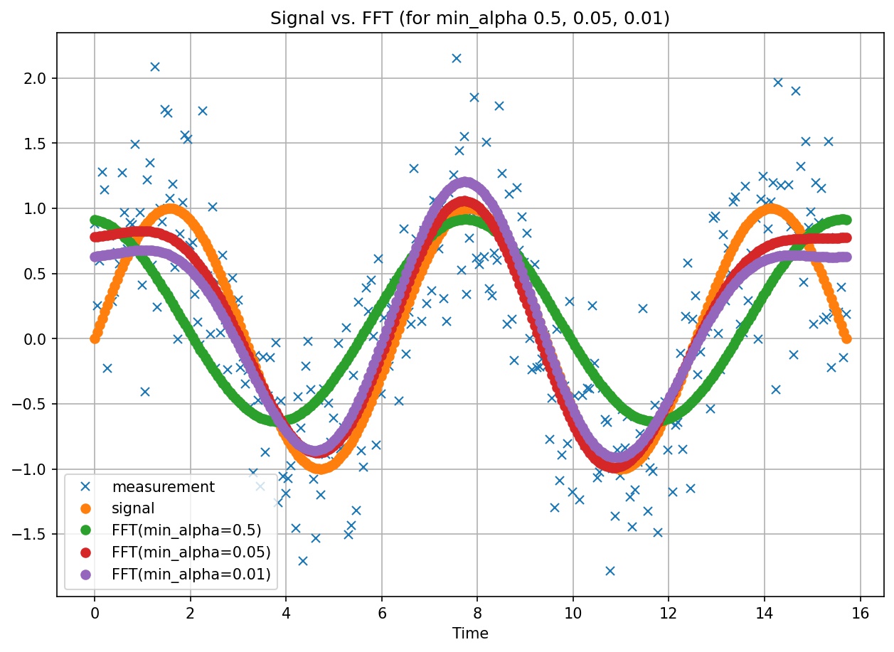
FFT signal extraction for varying values of min_alpha
Fast Fourier Transform is an algorithm that transforms a signal from time-domain to frequency-domain. FFT is applied to functions the same way PCA is applied to vector spaces.
The authors caution of Fourier’s analysis ability to equally fit noise. Hence, the authors provide us with a mechanism of preventing overfitting noise by means.
To prevent this overfitting problem, the authors provide the following solution. At every iteration of the algorithm, they scan all unused frequencies looking for the one that delivers the greatest decrease on the Ljung-Box statistic. The algorithm stops when the probability associated with the Ljung-Box statistic exceeds threshold min_alpha, or could not reduce by said threshold, as further scanning is unwarranted.
Implementation
Example
Locally Weighted Scatterplot Smoothing (LOWESS)
Overview
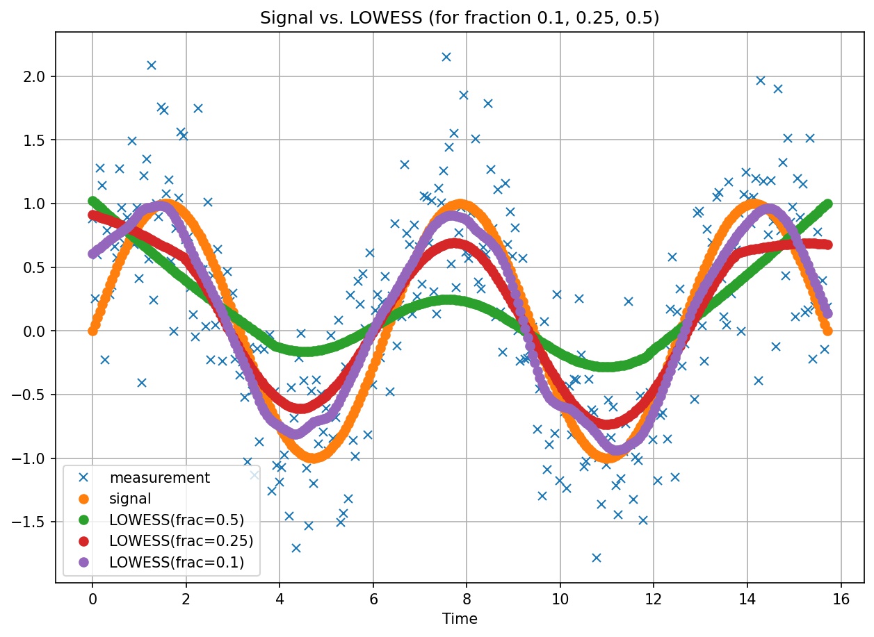
LOWESS signal extraction for varying values of fraction
LOWESS fits weighted linear regressions to localized subsets of data in order to filter noise by point.
The parameter fraction indicates to the LOWESS algorithm the fraction of data to use for the fit. As can be seen on the above plot, the smaller the value of fraction, the better the fit (e.g. frac=0.1) to the original signal, at an added cost of stability the bumps in the generated signal.
Implementation
Tip
Our LOWESS implementation is a wrapper around the same algorithm provided by statsmodels. See implementation here.
Example
Research Notebook
The following research notebook can be used to better understand noise reduction methods.