Visualising Graphs
This section outlines how to create visualisations using the helper function from visualisations.py. The helper functions streamline the process of constructing the MST and DashGraph objects. This is the recommended way to create visualisations, unless you would like to pass in a custom matrix.
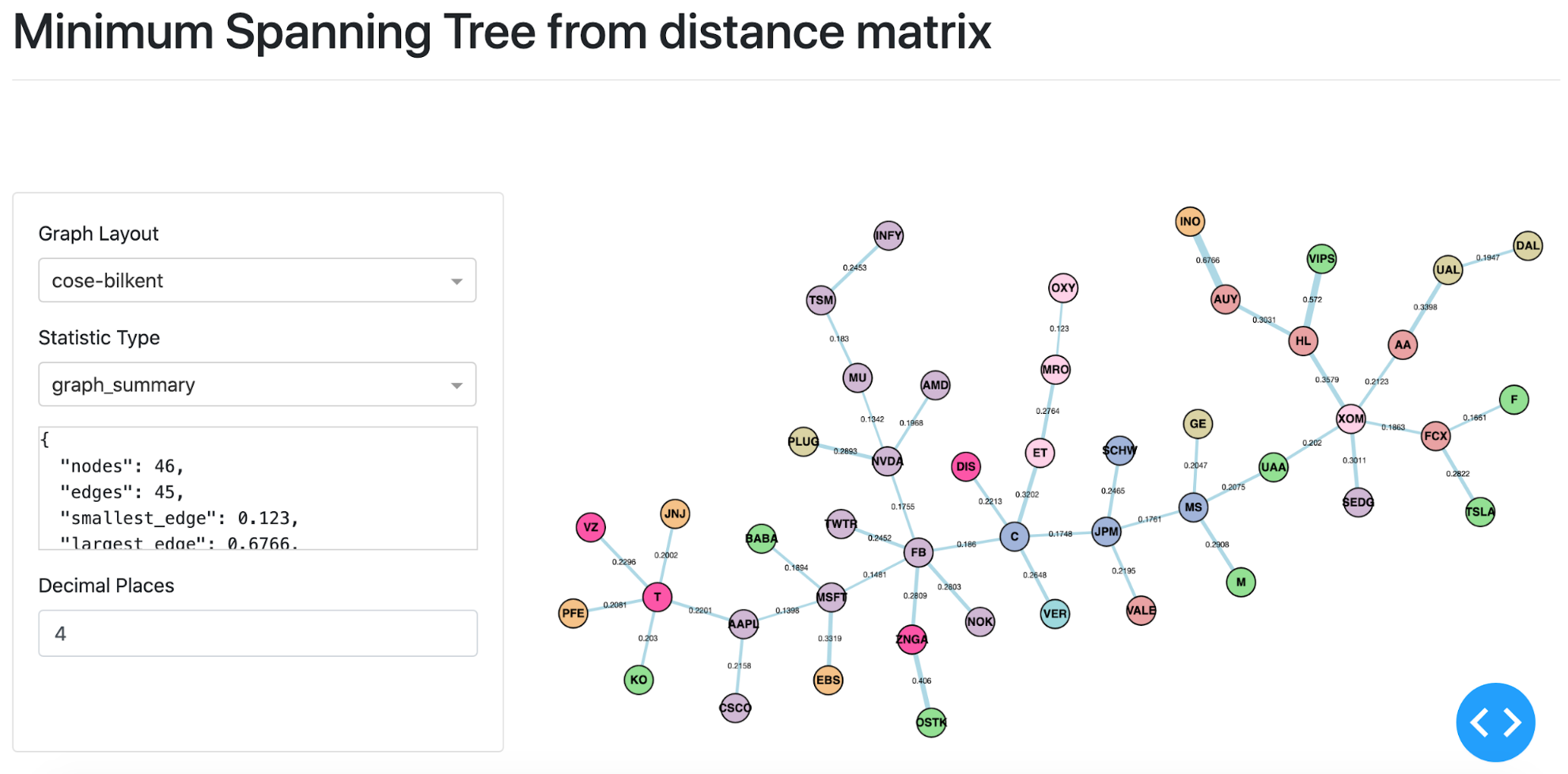
MST visualisation based on stock price data form 18th February 2020 until the 24th of March 2020.
To pass in a custom matrix, you must construct MST and DashGraph directly. Please refer to the MST with Custom Matrix section in the MST part of the documentation.
Creating Visualisations
The code snippet below shows how to create a MST visualisation and run the Dash server using the generate_mst_server method.
The code snippet creates a distance matrix, inputs it into the MST class, which is passed to the DashGraph class.
To input a custom matrix, you can use the MST class constructor instead.
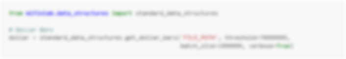
Example Code
Input File Format
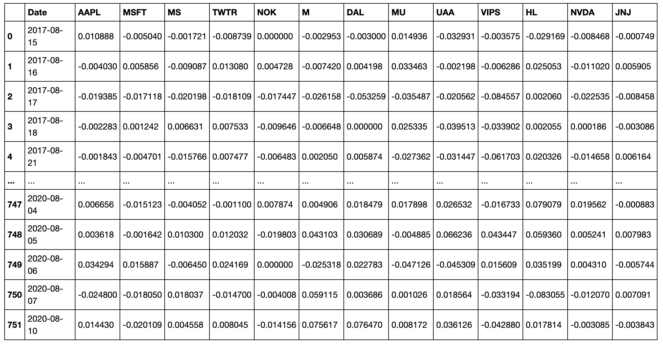
When using the generate_mst_server method as in the example above, the input file should be a time series of log returns. An example of the csv when imported as a dataframe (as the log_return_dataframe in the above example), is shown below.
The formula to calculate the log returns from OHLCV data is given as:
Let \(n\) be the number of assets, \(P_i(t)\) be price \(t\) of asset \(i\) and \(r_i(t)\) be the log-return at time \(t\) of asset \(i\):
For a more detailed explanation, please refer to Correlation-Based Metrics section, as it describes the measures in more detail.
Creating ALMST Visualisations
Similar to creating MST visualisations, you can use the generate_almst_server to create the ALMST server instead of the MST server. However, the input parameters and the output server are the same for the ALMST class. Both ALMST and MST are subclasses of the parent class Graph.
The optional parameters such as colours, node sizes, and the Jupyter notebook mode are set in the same way as the MST.
Comparing ALMST and MST
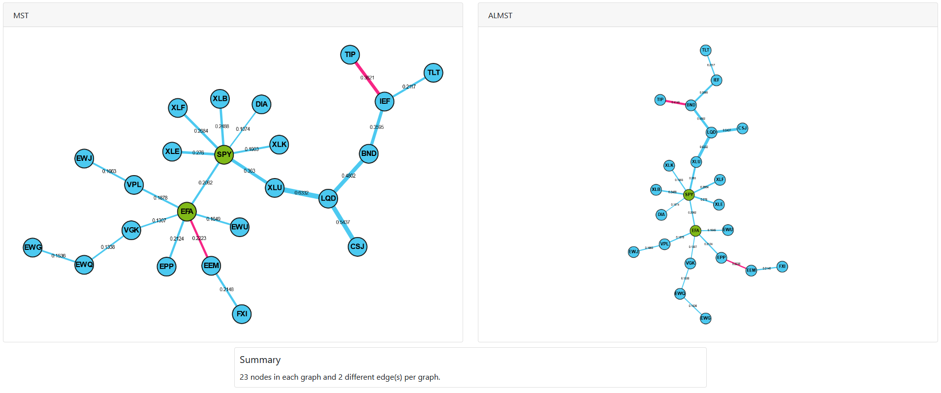
In order to create a dual interface to compare both the ALMST and MST, we can use the generate_mst_almst_comparison method with the ALMST and MST as the input.
Implementation
The generate_mst_server and generate_almst_server methods construct the server, ready to be run. It streamlines the process of creating a
MST or ALMST respectively, and DashGraph object, and various optional parameters can be passed.
Jupyter Notebook
An additional parameter jupyter=True must be passed to create a JupyterDash object instead of a Dash object. To run the server inside the notebook, pass the mode inline, external or jupyterlab to the method run_server. The Jupyter Dash library is used to provide this functionality. To utilise within Jupyter Notebook, replace:
With:
Adding Colours
The colours can be added by passing a dictionary of group name to list of node names corresponding to the nodes input. You then pass the dictionary as an argument.
Adding Sizes
The sizes can be added in a similar manner, via a list of numbers which correspond to the node indexes. The UI of the graph will then display the nodes indicating the different sizes.
MST Algorithm
Kruskal’s algorithms is used as a default. To use Prim’s algorithm instead, pass the parameter mst_algorithm=’prim’ into the generate_mst_server method.
Distance Matrix
The generate_mst_server method takes in a dataframe of log returns. A Pearson correlation matrix is then calculated from the log returns dataframe. The correlation matrix is the input to the method get_distance_matrix from the Codependence module. The valid distance matrix types are ‘angular’, ‘abs_angular’, and ‘squared_angular’. Explanations on the different types of distance matrices can be found on the Codependence module section.
Ranking Nodes by Centrality
For a PMFG graph, you can create a centrality ranking of the nodes. The ranking is based on the sum of 6 centrality measures, detailed below, all of which call methods from NetworkX centrality methods.
An example for ranking of PMFG is shown below.
The ranking returns an ordered list of tuples with the node name as the key and ranking as the value. The formula for the ranking is defined as:
Where \(C_{D}^w\) is the weighted degree, and \(C_{D}^u\) is the degree for the unweighted graph. The factors included are: Degree (D), Betweenness Centrality (BC), Eccentricity (E), Closeness Centrality (C), Second Order Centrality (SO) and Eigenvector Centrality (EC).
The Second Order Centrality (SO) is divided, as the output values would have a disproportionately large impact on the ranking.