Note
The following documentation closely follows the work by Marti et al.: Exploring and measuring non-linear correlations: Copulas, Lightspeed Transportation and Clustering.
The initial implementation was taken from the blog post by Gautier Marti: Measuring non-linear dependence with Optimal Transport.
Optimal Transport
As described by Gautier Marti here.:
“The basic idea of the optimal copula transport dependence measure is rather simple. It relies on leveraging:
Copulas, which are distributions encoding fully the dependence between random variables.
A geometrical point of view: Where does the empirical copula stand in the space of copulas? In particular, how far is it from reference copulas such as the Fréchet–Hoeffding copula bounds (copulas associated to comonotone, countermonotone, independent random variables)?”
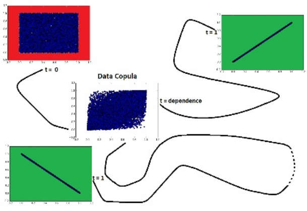
Dependence is measured as the relative distance from independence to the nearest target-dependence: comonotonicity or countermonotonicity. (Blog post by Gautier Marti)
“With this geometric view:
It is rather easy to extend this novel dependence measure to alternative use cases (e.g. by changing the reference copulas).
It can also allow to look for specific patterns in the dependence structure (generalization of conditional correlation).
With this optimal copula transport dependence tool, one can look for answers to, for example:
“Which pair of assets having \(\rho = 0.7\) correlation has the nearest copula to the Gaussian one?”
“Which pairs of assets are both positively and negatively correlated?”
“Which assets occur extreme variations while those of others are relatively small, and conversely?”
“Which pairs of assets are positively correlated for small variations but uncorrelated otherwise?”
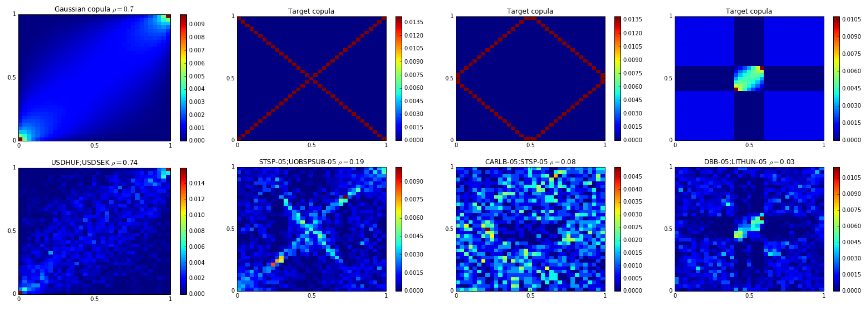
Target copulas (simulated or handcrafted) and their respective nearest copulas which answer questions A,B,C,D. (Marti et al. 2016)
Tip
For an example comparing the behaviour of Optimal Copula Transport dependence to Pearson’s correlation, Spearman’s rho, and Kendall tau distance, please read this blog post by Gautier Marti.
Note
Underlying Literature
The following sources elaborate extensively on the topic:
Exploring and measuring non-linear correlations: Copulas, Lightspeed Transportation and Clustering by Marti, G., Andler, S., Nielsen, F. and Donnat, P.
Optimal Copula Transport dependence
According to the description of the method from the original paper by Marti et al.:
The idea of the approach is to “target specific dependence patterns and ignore others. We want to target dependence which are relevant to such or such problem, and forget about the dependence which are not in the scope of the problems at hand, or even worse which may be spurious associations (pure chance or artifacts in the data).”
The proposed codependence coefficient “can be parameterized by a set of target-dependences, and a set of forget-dependences. Sets of target and forget dependences can be built using expert hypotheses, or by leveraging the centers of clusters resulting from an exploratory clustering of the pairwise dependences. To achieve this goal, we will leverage three tools: copulas, optimal transportation, and clustering.”
“Optimal transport is based on the underlying theory of the Earth Mover’s Distance. Until very recently, optimal transportation distances between distributions were not deemed relevant for machine learning applications since the best computational cost known was super-cubic to the number of bins used for discretizing the distribution supports which grows itself exponentially with the dimension. A mere distance evaluation could take several seconds!”
“Copulas and optimal transportation are not yet mainstream tools, but they have recently gained attention in machine learning, and several copula-based dependence measures have been proposed for improving feature selection methods”.
“Copulas are functions that couple multivariate distribution functions to their univariate marginal distribution functions”.
In this implementation, only bivariate copulas are considered, as higher dimensions would cost a high computational burden. But most of the results and the methodology presented hold in the multivariate setting.
Note
Theorem 1 (Sklar’s Theorem) Let \(X = (X_i, X_j)\) be a random vector with a joint cumulative distribution function \(F\) , and having continuous marginal cumulative distribution functions \(F_i, F_j\) respectively. Then, there exists a unique distribution \(C\) such that \(F(X_i, X_j) = C(F_i(X_i), F_j(X_j))\) . \(C\) , the copula of \(X\) , is the bivariate distribution of uniform marginals \(U_i, U_j := F_i(X_i), F_j(X_j)\)
“Copulas are central for studying the dependence between random variables: their uniform marginals jointly encode all the dependence. They allow to study scale-free measures of dependence and are invariant to monotonous transformations of the variables. Some copulas play a major role in the measure of dependence, namely \(\mathcal{W}\) and \(\mathcal{M}\) the Frechet-Hoeffding copula bounds, and the independence copula \(\Pi (u_i,u_j) = u_i u_j\) “.
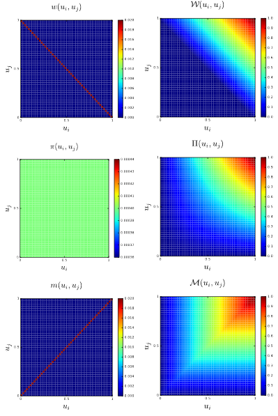
Copulas measure (left column) and cumulative distribution function (right column) heatmaps for negative dependence (first row), independence (second row), i.e. the uniform distribution over \([0, 1]^2\), and positive dependence (third row) (Marti et al. 2016)
Note
Proposition 1 (Frechet-Hoeffding copula bounds) For any copula \(C: [0, 1]^2 \rightarrow [0, 1]\) and any \((u_i, u_j) \in [0, 1]^2\) the following bounds hold:
where \(\mathcal{W} (u_i, u_j) = max \{u_i + u_j − 1, 0 \}\) is the copula for countermonotonic random variables and \(\mathcal{M} (u_i, u_j) = min \{ u_i, u_j \}\) is the copula for comonotonic random variables.
“Notice that when working with empirical data, we do not know a priori the margins \(F_i\) for applying the probability integral transform \(U_i := F_i(X_i)\) . Deheuvels has introduced a practical estimator for the uniform margins and the underlying copula, the empirical copula transform”.
Note
Definition 1 (Empirical Copula Transform) Let \((X^t_i, X^t_j), t = 1, ..., T\) , be \(T\) observations from a random vector \((X_i, X_j)\) with continuous margins. Since one cannot directly obtain the corresponding copula observations \((U^t_i, U^t_j) := (F_i(X^t_i), F_j(X^t_j))\) , where \(t = 1, ..., T\) , without knowing a priori \(F_i\) , one can instead estimate the empirical margins \(F^T_i(x) = \frac{1}{T} \sum^T_{t=1} I(X^t_i \le x)\) , to obtain the \(T\) empirical observations \((\widetilde{U}^t_i, \widetilde{U}^t_j) := (F^T_i(X^t_i), F^T_j(X^t_j))\) . Equivalently, since \(U^t_i = R^t_i / T, R^t_i\) being the rank of observation \(X^t_i\) , the empirical copula transform can be considered as the normalized rank transform.
“The idea of optimal transport is intuitive. It was first formulated by Gaspard Monge in 1781 as a problem to efficiently level the ground: Given that work is measured by the distance multiplied by the amount of dirt displaced, what is the minimum amount of work required to level the ground? Optimal transport plans and distances give the answer to this problem. In practice, empirical distributions can be represented by histograms.
Let \(r, c\) be two histograms in the probability simplex \(\sum_m = \{x \in R^m_+ : x^T 1_m = 1\}\) . Let \(U(r, c) = \{ P \in R^{m × m}_+ | P1_m = r, P^T 1_m = c\}\) be the transportation polytope of \(r\) and \(c\) , that is the set containing all possible transport plans between \(r\) and \(c\) “.
Note
Definition 2 (Optimal Transport) Given a \(m × m\) cost matrix \(M\), the cost of mapping \(r\) to \(c\) using a transportation matrix \(P\) can be quantified as \(\langle P, M \rangle _F\) , where \(\langle ·, ·\rangle _F\) is the Frobenius dot-product. The optimal transport between \(r\) and \(c\) given transportation cost \(M\) is thus:
“Whenever \(M\) belongs to the cone of distance matrices, the optimum of the transportation problem \(d_M(r, c)\) is itself a distance.
Using the optimal transport distance between copulas, we now propose a dependence coefficient which is parameterized by two sets of copulas: target copulas and forget copulas”.
Note
Definition 3 (Target/Forget Dependence Coefficient) Let \({C^−_l}_l\) be the set of forget-dependence copulas. Let \({C^+_k}_k\) be the set of target-dependence copulas. Let \(C\) be the copula of \((X_i, X_j)\) . Let \(d_M\) be an optimal transport distance parameterized by a ground metric \(M\) . We define the Target/Forget Dependence Coefficient as:
“Using this definition, we obtain:
It is known by risk managers how dangerous it can be to rely solely on a correlation coefficient to measure dependence. That is why we have proposed a novel approach to explore, summarize and measure the pairwise correlations which exist between variables in a dataset. The experiments show the benefits of the proposed method: It allows to highlight the various dependence patterns that can be found between financial time series, which strongly depart from the Gaussian copula widely used in financial engineering. Though answering dependence queries as briefly outlined is still an art, we plan to develop a rich language so that a user can formulate complex questions about dependence, which will be automatically translated into copulas in order to let the methodology provide these questions accurate answers”.
Implementation

Research Notebook
The following research notebook can be used to better understand the optimal copula transport dependence measure described above.