Information-driven bars are based on the notion of sampling a bar when new information arrives to the market. The two types of information-driven bars implemented are imbalance bars and run bars. For each type, tick, volume, and dollar bars are included.

For those new to the topic, it is discussed in the graduate level textbook: Advances in Financial Machine Learning, Chapter 2.

Warning

This is a very advanced financial data structure with very little to no academic papers written about them. Our team has analysed the statistical properties and its not clear to us how to use this structure.

We highly recommend that you read the literature, plus that of microstructural features before committing to this data structure.

Imbalance Bars¶

2 types of imbalance bars are implemented in MlFinLab:

Expected number of ticks, defined as EMA (book implementation)

Constant number of expected number of ticks.

The Generation Algorithm¶

Let’s discuss the generation of imbalance bars on an example of volume imbalance bars. As it is described in Advances in Financial Machine Learning book:

First let’s define what is the tick rule:

\[\begin{split}b_t = \begin{cases} b_{t-1},\;\;\;\;\;\;\;\;\;\; \Delta p_t \mbox{=0} \\ |\Delta p_t| / \Delta p_{t},\;\;\; \Delta p_t \neq\mbox{0} \end{cases}\end{split}\]

For any given \(t\), where \(p_t\) is the price associated with \(t\) and \(v_t\) is volume, the tick rule \(b_t\) is defined as:

Tick rule is used as a proxy of trade direction, however, some data providers already provide customers with tick direction, in this case we don’t need to calculate tick rule, just use the provided tick direction instead.

Cumulative volume imbalance from \(1\) to \(T\) is defined as:

\[\theta_t = \sum_{t=1}^T b_t*v_t`\]

Where \(T\) is the time when the bar is sampled.

Next we need to define \(E_0[T]\) as the expected number of ticks, the book suggests to use a exponentially weighted moving average (EWMA) of the expected number of ticks from previously generated bars. Let’s introduce the first hyperparameter for imbalance bars generation: num_prev_bars which corresponds to the window used for EWMA calculation.

Here we face the problem of the first bar’s generation, because we don’t know the expected number of ticks upfront. To solve this we introduce the second hyperparameter: expected_num_ticks_init which corresponds to initial guess for expected number of ticks before the first imbalance bar is generated.

Bar is sampled when:

\[|\theta_t| \geq E_0[T]*[2v^+ - E_0[v_t]]\]

To estimate (expected imbalance) we simply calculate the EWMA of volume imbalance from previous bars, that is why we need to store volume imbalances in an imbalance array, the window for estimation is either expected_num_ticks_init before the first bar is sampled, or expected number of ticks(\(E_0[T]\)) * num_prev_bars when the first bar is generated.

Note that when we have at least one imbalance bar generated we update \(2v^+ - E_0[v_t]\) only when the next bar is sampled and not on every trade observed

Algorithm Logic¶

Now that we have understood the logic of the imbalance bar generation, let’s understand the process in further detail.

# Pseudo code
num_prev_bars = 3
expected_num_ticks_init = 100000
expected_num_ticks = expected_num_ticks_init
cum_theta = 0
num_ticks = 0
imbalance_array = []
imbalance_bars = []
bar_length_array = []

for row in data.rows:
    # Track high, low,c lose, volume info
    num_ticks += 1
    tick_rule = get_tick_rule(price, prev_price)
    volume_imbalance = tick_rule * row['volume']
    imbalance_array.append(volume_imbalance)
    cum_theta += volume_imbalance
    if len(imbalance_bars) == 0 and len(imbalance_array) >= expected_num_ticks_init:
        expected_imbalance = ewma(imbalance_array, window=expected_num_ticks_init)

    if abs(cum_theta) >= expected_num_ticks * abs(expected_imbalance):
        bar = form_bar(open, high, low, close, volume)
        imbalance_bars.append(bar)
        bar_length_array.append(num_ticks)
        cum_theta, num_ticks = 0, 0
        expected_num_ticks = ewma(bar_lenght_array, window=num_prev_bars)
        expected_imbalance = ewma(imbalance_array, window = num_prev_bars*expected_num_ticks)

Note that in algorithm pseudo-code we reset \(\theta_t\) when bar is formed, in our case the formula for \(\theta_t\) is:

\[\theta_t = \sum_{t=t^*}^T b_t*v_t\]

Let’s look at dynamics of \(|\theta_t|\) and \(E_0[T] * |2v^+ - E_0[v_t]|\) to understand why we decided to reset \(\theta_t\) when a bar is formed. The following figure highlights the dynamics when theta value is reset:

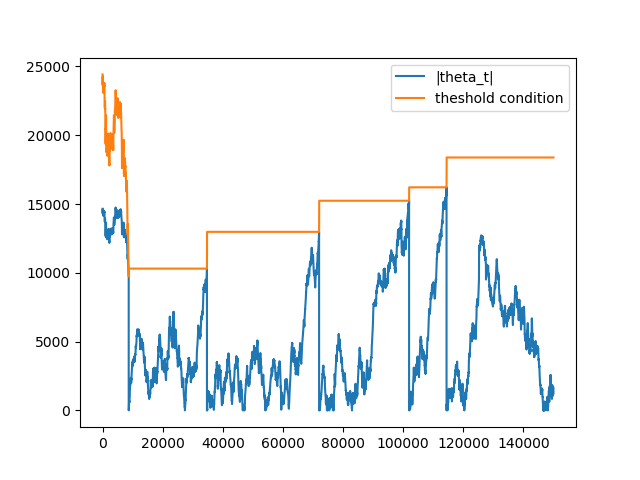
Note that on the first set of ticks, the threshold condition is not stable. Remember, before the first bar is generated, the expected imbalance is calculated on every tick with window = expected_num_ticks_init, that is why it changes with every tick. After the first bar was generated both expected number of ticks (\(E_0[T]\)) and expected volume imbalance (\(2v^+ - E_0[v_t]\)) are updated only when the next bar is generated

When theta is not reset:

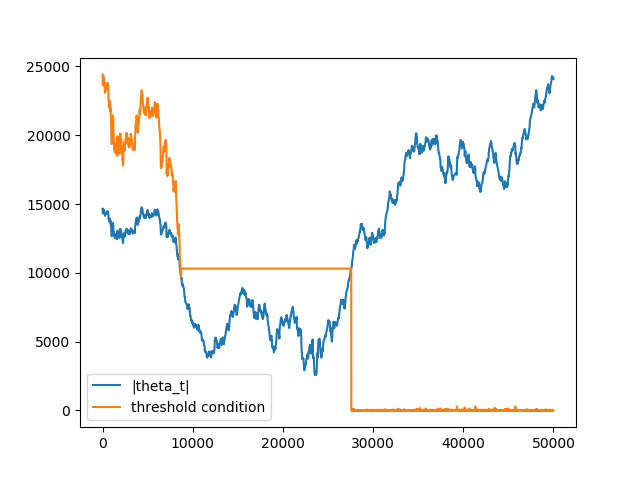
The reason for that is due to the fact that theta is accumulated when several bars are generated theta value is not reset \(\Rightarrow\) condition is met on small number of ticks \(\Rightarrow\) length of the next bar converges to 1 \(\Rightarrow\) bar is sampled on the next consecutive tick.

The logic described above is implemented in the MlFinLab package under ImbalanceBars

Implementations¶

There are 2 different implementations which have been discussed in the previous section.

EMA Version¶

Tick Bars¶

Volume Bars¶

Dollar Bars¶

Constant Version¶

Tick Bars¶

Volume Bars¶

Dollar Bars¶

Example¶

Research Notebooks¶

The following research notebooks can be used to better understand the previously discussed data structures.

Presentation Slides¶

References¶

de Prado, M.L., 2018. Advances in financial machine learning. John Wiley & Sons.