Fractionally Differentiated Features
Note
We’ve further improved the model described in Advances in Financial Machine Learning by prof. Marcos Lopez de Prado to speed up the execution time.
Starting from MlFinLab version 1.5.0 the execution is up to 10 times faster compared to the models from version 1.4.0 and earlier. (The speed improvement depends on the size of the input dataset)
One of the challenges of quantitative analysis in finance is that time series of prices have trends or a non-constant mean. This makes the time series is non-stationary. A non-stationary time series are hard to work with when we want to do inferential analysis based on the variance of returns, or probability of loss.
Many supervised learning algorithms have the underlying assumption that the data is stationary. Specifically, in supervised learning, one needs to map hitherto unseen observations to a set of labeled examples and determine the label of the new observation.
According to Marcos Lopez de Prado: “If the features are not stationary we cannot map the new observation to a large number of known examples”. Making time series stationary often requires stationary data transformations, such as integer differentiation. These transformations remove memory from the series. The method proposed by Marcos Lopez de Prado aims to make data stationary while preserving as much memory as possible, as it’s the memory part that has predictive power.
Fractionally differentiated features approach allows differentiating a time series to the point where the series is stationary, but not over differencing such that we lose all predictive power.
Note
Underlying Literature
The following sources elaborate extensively on the topic:
Advances in Financial Machine Learning, Chapter 5 by Marcos Lopez de Prado. Describes the motivation behind the Fractionally Differentiated Features and algorithms in more detail
Fixed-width Window Fracdiff
The following description is based on Chapter 5 of Advances in Financial Machine Learning:
Using a positive coefficient \(d\) the memory can be preserved:
where \(X\) is the original series, the \(\widetilde{X}\) is the fractionally differentiated one, and the weights \(\omega\) are defined as follows:
“When \(d\) is a positive integer number, \(\prod_{i=0}^{k-1}\frac{d-i}{k!} = 0, \forall k > d\), and memory beyond that point is cancelled.”
Given a series of \(T\) observations, for each window length \(l\), the relative weight-loss can be calculated as:
The weight-loss calculation is attributed to a fact that “the initial points have a different amount of memory” ( \(\widetilde{X}_{T-l}\) uses \(\{ \omega \}, k=0, .., T-l-1\) ) compared to the final points ( \(\widetilde{X}_{T}\) uses \(\{ \omega \}, k=0, .., T-1\) ).
With a defined tolerance level \(\tau \in [0, 1]\) a \(l^{*}\) can be calculated so that \(\lambda_{l^{*}} \le \tau\) and \(\lambda_{l^{*}+1} > \tau\), which determines the first \(\{ \widetilde{X}_{t} \}_{t=1,...,l^{*}}\) where “the weight-loss is beyond the acceptable threshold \(\lambda_{t} > \tau\) .”
Without the control of weight-loss the \(\widetilde{X}\) series will pose a severe negative drift. This problem is corrected by using a fixed-width window and not an expanding one.
With a fixed-width window, the weights \(\omega\) are adjusted to \(\widetilde{\omega}\) :
Therefore, the fractionally differentiated series is calculated as:
for \(t = T - l^{*} + 1, ..., T\)
The following graph shows a fractionally differenced series plotted over the original closing price series:
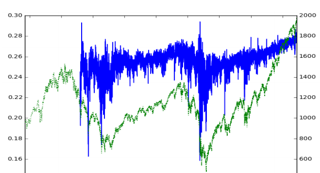
Fractionally differentiated series with a fixed-width window (Lopez de Prado 2018)
Tip
A deeper analysis of the problem and the tests of the method on various futures is available in the Chapter 5 of Advances in Financial Machine Learning.
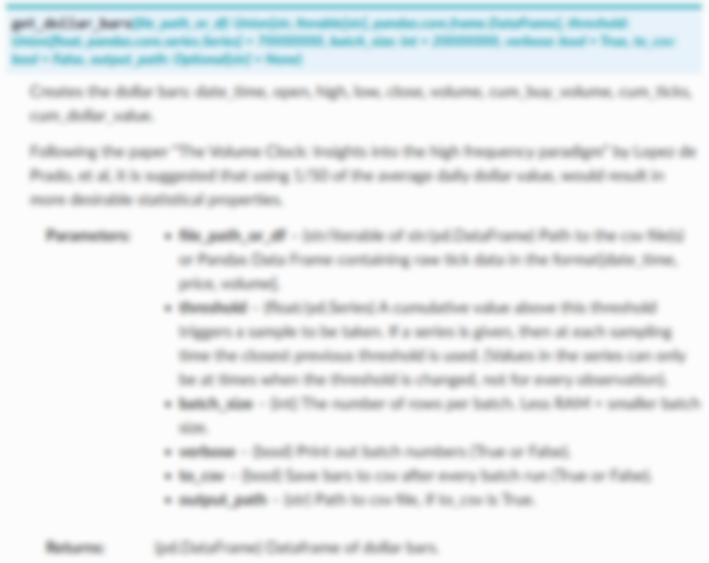
Implementation
The following function implemented in MlFinLab can be used to derive fractionally differentiated features.
Stationarity With Maximum Memory Representation
The following description is based on Chapter 5 of Advances in Financial Machine Learning:
Applying the fixed-width window fracdiff (FFD) method on series, the minimum coefficient \(d^{*}\) can be computed. With this \(d^{*}\) the resulting fractionally differentiated series is stationary. This coefficient \(d^{*}\) quantifies the amount of memory that needs to be removed to achieve stationarity.
If the input series:
is already stationary, then \(d^{*}=0\).
contains a unit root, then \(d^{*} < 1\).
exhibits explosive behavior (like in a bubble), then \(d^{*} > 1\).
A case of particular interest is \(0 < d^{*} \ll 1\), when the original series is “mildly non-stationary.” In this case, although differentiation is needed, a full integer differentiation removes excessive memory (and predictive power).
The following grap shows how the output of a plot_min_ffd function looks.
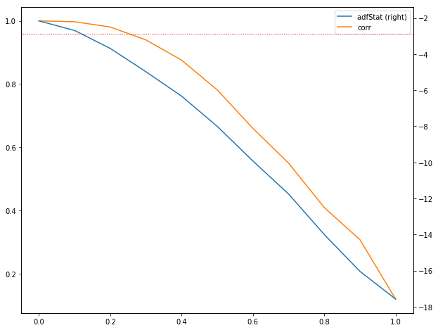
ADF statistic as a function of d
The right y-axis on the plot is the ADF statistic computed on the input series downsampled to a daily frequency.
The x-axis displays the d value used to generate the series on which the ADF statistic is computed.
The left y-axis plots the correlation between the original series ( \(d = 0\) ) and the differentiated series at various \(d\) values.
The horizontal dotted line is the ADF test critical value at a 95% confidence level. Based on where the ADF statistic crosses this threshold, the minimum \(d\) value can be defined.
The correlation coefficient at a given \(d\) value can be used to determine the amount of memory that was given up to achieve stationarity. (The higher the correlation - the less memory was given up)
According to Lopez de Prado:
“Virtually all finance papers attempt to recover stationarity by applying an integer differentiation \(d = 1\), which means that most studies have over-differentiated the series, that is, they have removed much more memory than was necessary to satisfy standard econometric assumptions.”
Tip
An example on how the resulting figure can be analyzed is available in Chapter 5 of Advances in Financial Machine Learning.
Implementation
The following function implemented in MlFinLab can be used to achieve stationarity with maximum memory representation.
Example
Given that we know the amount we want to difference our price series, fractionally differentiated features, and the minimum d value that passes the ADF test can be derived as follows:
Research Notebook
The following research notebook can be used to better understand fractionally differentiated features.
Research Article
Presentation Slides