First Generation Models
Market microstructure studies the process and outcomes of exchanging assets under explicit trading rules - O’Hara, 1995
Microstructural datasets include primary information about the auctioning process, like order cancellations, double action book, queues, partial fills, aggressor side, corrections, and replacements. These datasets provide researchers with the ability to understand how market participants conceal and reveal their true preferences, making them incredibly useful for engineering features of an ML model.
This module concerns itself with the so-called “first generation” of microstructural models and a series of transformations of their outputs - namely:
The Tick Rule
The Roll Model
Fractional Differentiation
Wald-Wolfowitz Runs Randomness
Entropy Measures
It also includes a generate_feature_matrix function, which allows for the convenient application of all of the features contained in this module to a dataset of ticks on a rolling basis, creating a ready-to-use input dataframe for an ML model
Note
Underlying Literature
The following sources elaborate extensively on the topic:
Advances in Financial Machine Learning, Chapter 19, Section 3 by Marcos Lopez de Prado. Describes the emergence and modern day uses of the first generation of microstructural features in more detail
The Tick Rule
The following description is based on Section 19.3.1 of Advances in Financial Machine Learning:
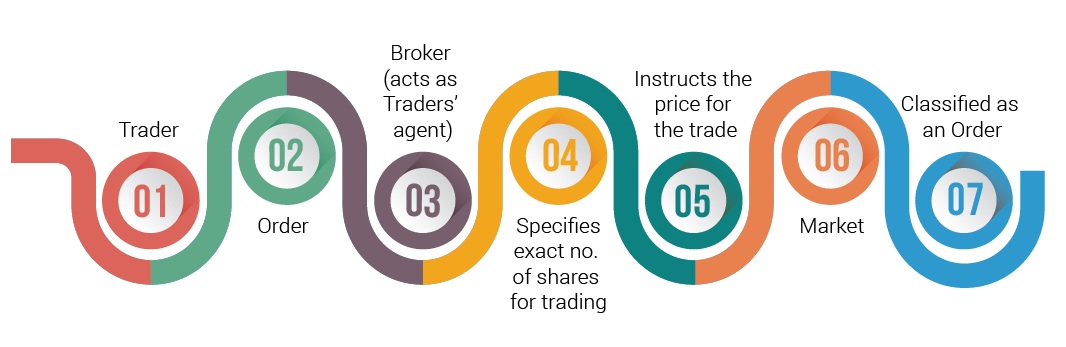
In a double auction book, quotes are placed for selling a security at various price levels or for buying a security at various price levels. Offer prices always exceed bids prices, because otherwise there would be an instant match. A trade occurs whenever a buyer matches an offer or a seller matches a bid. Every trade has a buyer and a seller, but only one side initiates the trade.
The Tick Rule is an algorithm used to determine a trade’s aggressor side. A buy-initiated trade is labeled (1) and a sell-initiated trade is labeled (-1), according to the following logic:
where \(p_{t}\) is the price of the trade indexed by \(t = 1,...T\), and \(b_{0}\) is arbitrarily set to 1.
The Roll Model
The following description is based on Section 19.3.2 of Advances in Financial Machine Learning:
The Roll Model (1984) provides market microstructure model that aims at estimating the effective bid-ask spread of a security from observed transaction prices. That said, the Roll model does not include any information on the underlying bid-ask price quotes and order flow.
Consider a mid-price series \({p_{t}}\), where prices follow a Random Walk with no drift as follows:
hence price changes \(\Delta m_{t} = m_{t} - m_{t-1}\) are independently and identically drawn from a Normal distribution:
The observed prices, \({p_{t}}\), are the result of sequential trading against the bid-ask spread:
where \(c\) is half the bid-ask spread, and \(b_{t} \in\{-1, 1\}\) is the aggressor side. The Roll model assumes that buys and sells are equally likely, \(P\left[b_{t}=1\right]=P\left[b_{t}=-1\right]=\frac{1}{2}\), serially independent, \(E\left[b_{t}b_{t-1}\right]=0\), and independent from the noise, \(E\left[b_{t}u_{t}\right]=0\). Given these assumptions, Roll derives the values of \(c\) and \(\sigma_{u}^2\) as follows:
resulting in:
As a result, we can conclude that the bid-ask spread is a function of the serial covariance of price changes, and the true (unobserved) price’s noise, excluding microstructural noise, is a function of the observed noise and the serial covariance of price changes.
Feature Transformations
As previously mentioned, there are many transformations that can be applied to the trade classifications yielded by the Tick Rule that make for interesting feature inputs to an ML model. The transformations contained in this module include the Wald-Wolfowitz Runs test to the classification series to determine how random the classifications are, fractional differencing of the classification series to achieve stationarity while simultaneously preserving a high degree of information, and various entropy measures that determine the amount of information contained in the classification sequence.
Fractional Differentiation
For a detailed explanation of fractional differentiation and why it’s useful for machine learning in finance, please consult Fractionally Differentiated Features, of the MLFinLab documentation
In the context of microstructural features, the cumulative sum of tick-rule generated trade classifications can be fractionally differenced in order to produce an information rich time series that is also stationary (as determined by the Augmented Dickey-Fuller test)
Wald-Wolfowitz Runs Randomness
The Wald–Wolfowitz runs test is a statistical test that determines whether or not a two-valued data sequence is random. The test can be used to test the hypothesis that the elements of a sequence are mutually independent. In the context of microstructural features, the p-value of a Wald-Wolfowitz test applied to a window of classifications can be used to determine if there have been more sell-initiated or buy-initiated trades for a given security, which in turn sheds light on a security’s liquidity


Entropy Measures
For a detailed explanation of the entropy measures listed below, their implementations, and why they are useful for machine learning in finance, please consult Entropy Measures, of the MLFinLab documentation
Shanon Entropy
Plug-in (or Maximum Likelihood) Entropy
Lempel-Ziv Entropy
Kontoyiannis Entropy
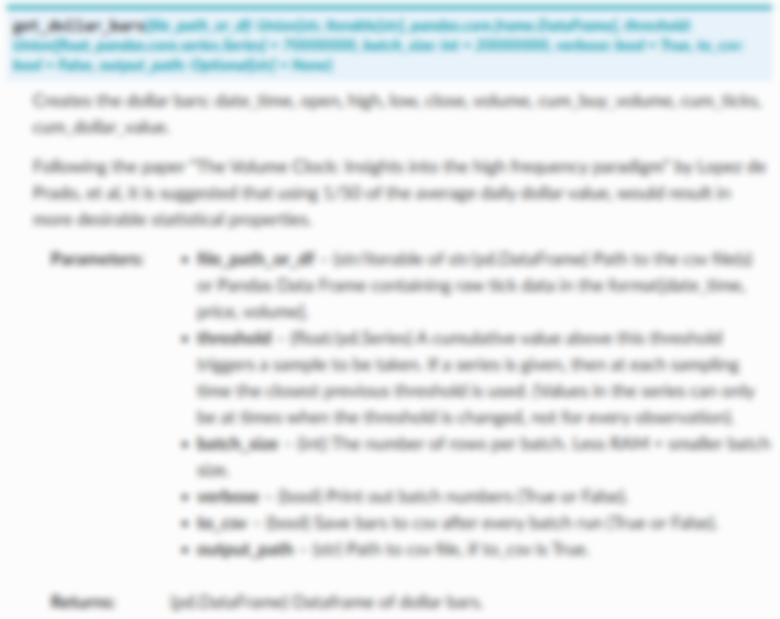
The Feature Matrix
The feature matrix is simply a dataframe that contains the application of all of the functions in this module and the Entropy Measures module applied to a tick bar dataset using a rolling window specified by the user (e.g. 5 ticks)
To best use this function, we first recommend using the fractional_differencing function on its own in order to best calibrate the differencing amount and differencing threshold that will be required as inputs to this function
Research Notebook
The following research notebook can be used to better understand the so-called “first generation” of microstructural models and the series of transformations of their outputs covered in this module: