Correlated Random Walks
Being able to discriminate random variables both on distribution and dependence on time series is motivated by the study of financial assets returns. The authors proposed a distance metric (GNPR) that “improves the performance of machine learning algorithms working on independent and identically distributed stochastic processes”.
As examined by the authors, there is a need for a generic representation of random variables for machine learning. They introduce a non-parametric approach to represent random variables that is able to split and detect different underlying distributions on a time series. This method is called the generic non-parametric representation (GNPR) approach, the authors have shown it separates distributions more effectively than other methods such as generic parametric representation (GPR), \(L_2\) distance, and distance correlation.
Note
The GNPR approach is described in our documentation, located in the Codependence by Marti section.
Note
Underlying Literature
The following sources elaborate extensively on the topic:
Toward a generic representation of random variables for machine learning by Donnat, P., Marti, G. and Very, P.
Time Series Generation with Different Distributions
In order to test and verify the efficiency of this approach, the authors provide a method to generate time series datasets. They are defined as \(N\) time series, each of length \(T\), which are subdivided into \(K\) correlation clusters, themselves subdivided into \(D\) distribution clusters.
If \(\textbf{W}\) is sampled from a normal distribution \(N(0, 1)\) of length \(T\), \((Y_k)_{k=1}^K\) is \(K\) i.i.d random distributions each of length \(T\), and \((Z_d^i)_{d=1}^D\); for \(i \leq i \leq N\) are independent random distributions of length \(T\), for \(i \leq i \leq N\) they define:
Where
\(\alpha_{d, i} = 1\), if \(i \equiv d - 1\) (mod \(D\)), 0 otherwise
\(\beta \in [0, 1]\)
\(\beta_{k, i} = \beta\), if \(\textit{ceil}(iK/N) = k\), 0 otherwise.
The authors show that even though the mean and the variance of the \((Y_k)\) and \((Z_d^i)\) distributions are the same and their variables are highly correlated, GNPR is able to successfully separate them into different clusters.
The distributions supported by default are:
Normal distribution (
np.random.normal)Laplace distribution (
np.random.laplace)Student’s t-distribution (
np.random.standard_t)
Implementation
To override the default distributions used to create the time series, the user must pass a list of the names of the distributions to use as the parameter dists_clusters.
The first value of this list is used to generate \((Y_k)_{k=1}^K\).
The available distributions are:
“normal” (
np.random.normal(0, 1))“normal_2” (
np.random.normal(0, 2))“laplace” (
np.random.laplace(0, 1 / np.sqrt(2)))“student-t” (
np.random.standard_t(3) / np.sqrt(3))
Example
The authors provide multiple parameters and distributions in their paper. \(N\) represents the normal distribution, \(L\) represents \(Laplace(0, 1/\sqrt{2})\), and \(S\) represents \(t-distribution(3)/\sqrt{3}\)
Clustering |
N |
T |
K |
D |
|
|
\(Y_k\) |
\(Z_1^i\) |
\(Z_2^i\) |
\(Z_3^i\) |
\(Z_4^i\) |
Distribution |
200 |
5000 |
1 |
4 |
0.1 |
0 |
\(N(0,1)\) |
\(N(0,1)\) |
\(L\) |
\(S\) |
\(N(0,2)\) |
Dependence |
200 |
5000 |
10 |
1 |
0.1 |
0.3 |
\(S\) |
\(S\) |
\(S\) |
\(S\) |
\(S\) |
Mix |
200 |
5000 |
5 |
2 |
0.1 |
0.3 |
\(N(0,1)\) |
\(N(0,1)\) |
\(S\) |
\(N(0,1)\) |
\(S\) |
The Distribution example generates a time series that has a global normal distribution, no correlation clustering, and 4 distribution clusters.
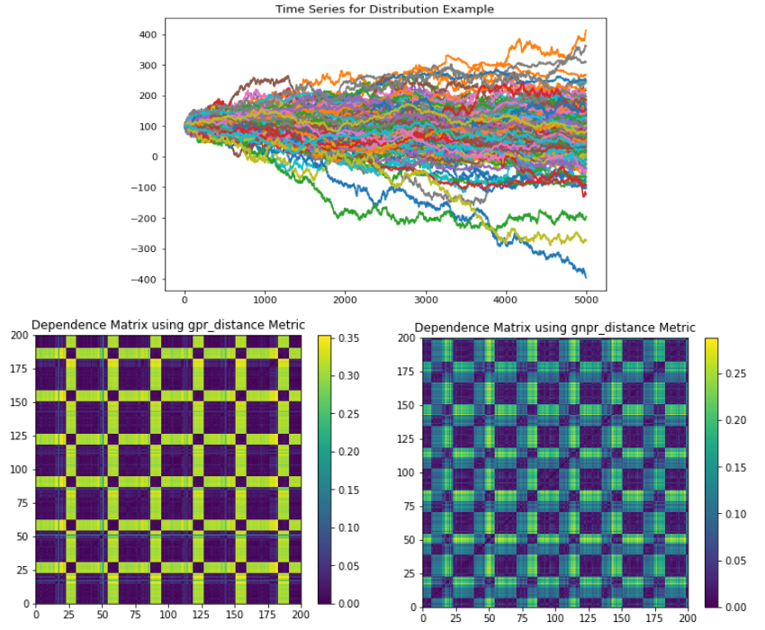
(Top) Time series plot. (Left) GPR codependence matrix. Only two apparent clusters are seen with no indication of a global embedded distribution. (Right). All 4 distributions clusters can be seen, as well as the global embedded distribution.
The Dependence example generates a time series that has a global normal distribution, 10 correlation clusters, and no distribution clusters.
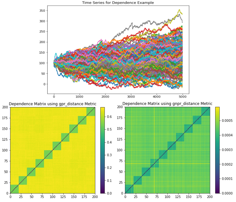
(Top) Time series plot. (Left) GPR codependence matrix. Only 10 correlation clusters are seen with no indication of a global embedded distribution. All 10 correlation clusters can be seen, as well as the global embedded distribution.
The Mix example generates a time series that has a global normal distribution, 5 correlation clusters, and 2 distribution clusters.
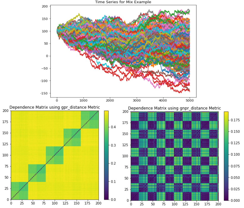
(Top) Time series plot. (Left) GPR codependence matrix. Only 5 correlation clusters are seen with no indication of a global embedded distribution. All 5 correlation clusters and 2 distribution clusters can be seen, as well as the global embedded distribution.
Research Notebook
The following research notebook can be used to better understand Correlated Random Walks.