Note
The following implementations and documentation, closely follows the lecture notes from Cornell University, by Marcos Lopez de Prado: Codependence (Presentation Slides).
Information Theory Metrics
We can gauge the codependence from the information theory perspective. In information theory, (Shannon’s) entropy is a measure of information (uncertainty). As described in the Cornell lecture slides, p.13 , entropy is calculated as:
Where \(X\) is a discrete random variable that takes a value \(x\) from the set \(S_{X}\) with probability \(p[x]\) .
In short, we can say that entropy is the expectation of the amount of information when we sample from a particular probability distribution or the number of bits to transmit to the target. So, if there is a correspondence between random variables, the correspondence will be reflected in entropy. For example, if two random variables are associated, the amount of information in the joint probability distribution of the two random variables will be less than the sum of the information in each random variable. This is because knowing a correspondence means knowing one random variable can reduce uncertainty about the other random variable.
This module presents two ways of measuring correspondence:
Mutual Information
Variation of Information
The following figure highlights how we can view the relationships of various information measures associated with correlated variables \(X\) and \(Y\) through the below figure. (Cornell lecture slides, p.24)
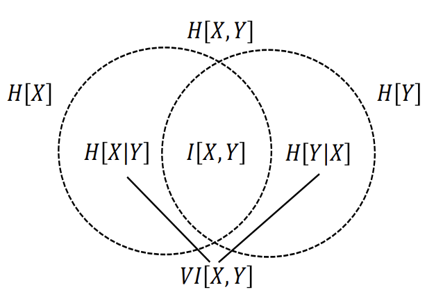
The correspondence between joint entropy, marginal entropies, conditional entropies, mutual information and variation of information (Lopez de Prado, 2020).
Note
Underlying Literature
The following sources elaborate extensively on the topic:
Codependence (Presentation Slides) by Marcos Lopez de Prado.
Mutual information is copula entropy by Ma, J. and Sun, Z.
Low bias histogram-based estimation of mutual information for feature selection by Hacine-Gharbi, A., Ravier, P., Harba, R. and Mohamadi, T.
A binning formula of bi-histogram for joint entropy estimation using mean square error minimization by Hacine-Gharbi, A. and Ravier, P.
Mutual Information
According to Lopez de Prado: “Mutual Information is defined as the decrease in uncertainty (or informational gain) in \(X\) that results from knowing the value of \(Y\). Mutual information is not a metric as it doesn’t satisfy the triangle inequality”. The properties of non-negativity and symmetry are satisfied. Mutual information is calculated as:
Mutual information has a grouping property:
where \((X, Y)\) is a joint distribution of \(X\) and \(Y\) .
It can also be normalized using a known upper boundary:
An alternative way of estimating the Mutual information is through using copulas. A link between Mutual information and copula entropy was presented in the paper by Ma, Jian & Sun, Zengqi. (2008). Mutual information is copula entropy.
A blog post by Gautier Marti includes descriptions of two alternative estimators of copula entropy:
First, estimate the copula (as a normalized ranking of the observations). Then apply the standard mutual information estimator on the normalized rankings of the observations.
First, estimate the copula (as a normalized ranking of the observations). Then and calculate the entropy of a copula. Estimator of the Mutual Information would be equal to negative copula entropy:
According to Gautier Marti, these two estimators have some advantages over the standard approach:
First, continuous marginals (think the distribution of returns of each stock) have a potentially unbounded support making it hard to bin properly.
Second, the discretization process to estimate the density used to compute the entropy, may introduce biases in the mutual information estimate due to a rather difficult and arbitrary binning of the support.
Using their copula \(C(X,Y)\), allows to bypass the estimation of the margins. The copula has compact support in \([0, 1]\), and its margins are uniform.
Alternative Mutual Information estimators are also available in the below function.
Implementation

Variation of Information
According to Lopez de Prado: “Variation of Information can be interpreted as the uncertainty we expect in one variable if we are told the value of another”. The variation of information is a true metric and satisfies the axioms from the introduction.
The upper bound of Variation of information is not firm as it depends on the sizes of the population which is problematic when comparing variations of information across different population sizes, as described in Cornell lecture slides, p.21
Implementation
Discretization
Both mutual information and variation of information are using random variables that are discrete. To use these tools for continuous random variables the discretization approach can be used.
For the continuous case, we can quantize the values to estimate \(H[X]\). Following the Cornell lecture slides, p.26 :
where the observed values \(\{x\}\) are divided into \(B_{X}\) bins of equal size \(\Delta_{X}\), \(\Delta_{X} = \frac{max\{x\} - min\{x\}}{B_{X}}\) , and \(f_{X}[x_{i}]\) is the frequency of observations within the i-th bin.
So, the discretized estimator of entropy is:
where \(N_{i}\) is the number of observations within the i-th bin, \(N = \sum_{i=1}^{B_{X}}N_{i}\) .
From the above equations, the size of the bins should be chosen. The results of the entropy estimation will depend on the binning. The works by Hacine-Gharbi et al. (2012) and Hacine-Gharbi and Ravier (2018) present optimal binning for marginal and joint entropy.
This optimal binning method is used in the mutual information and variation of information functions.
Implementation
Examples
The following example highlights how the various metrics behave under various variable dependencies:
Linear
Squared
\(Y = abs(X)\)
Independent variables
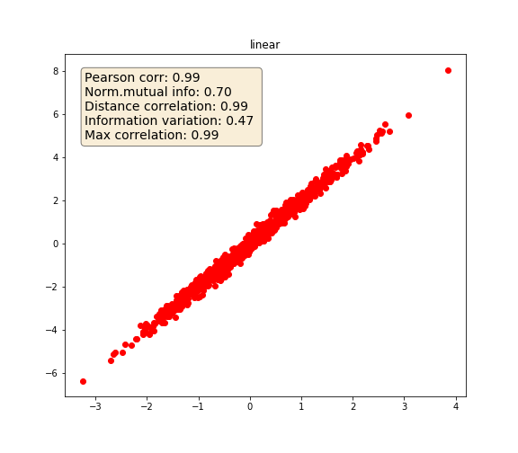
Linear
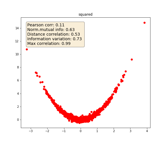
Squared
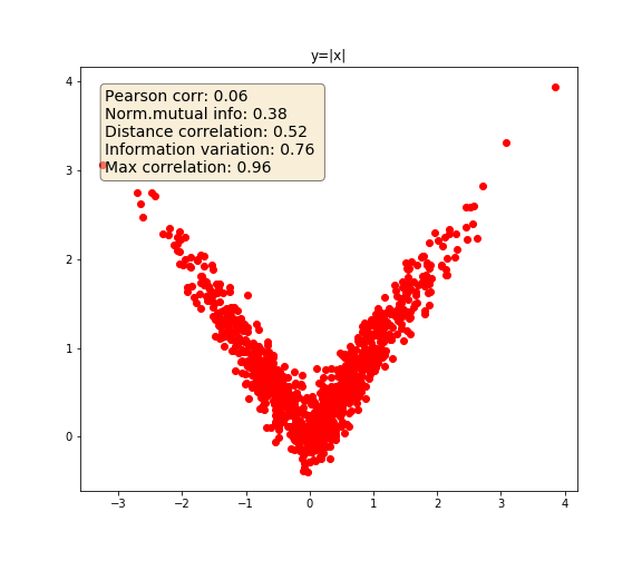
Absolute
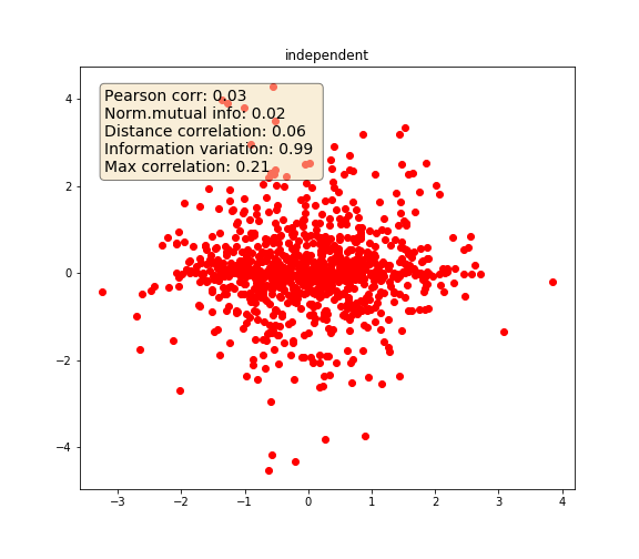
Independent